Repository navigation
problematic step() output: unstable instead of sinusoidal #384

Description
Activity
The system is ill-conditioned since the closed loop system has a pure imaginary pole => small numerical errors can generate problems.
The main problem in the
python-controlversion is that it is computing the time range for the step response differently. If you look closely at the units on the x axis for your first plot, you will see they go to 3e15 (!). If you give the step response an explicit time range, you get something that looks like Octave:from control.matlab import * import numpy as np import matplotlib.pyplot as plt Gp = tf(6, [1, 6, 11, 6]) Gc = 10 Gor = Gp*Gc/(1 + Gp*Gc) y, t = step(Gor, np.linspace(0, 10, 1000)) plt.plot(t, y)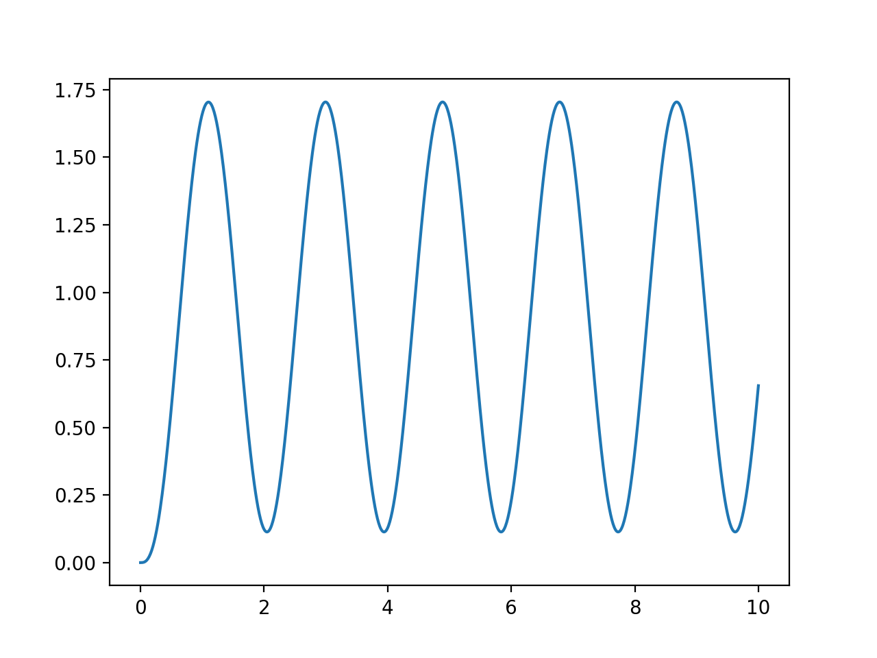
There is still a problem here to be fixed, which is the computation of the default time for the simulation in cases where there is a pure imaginary pole. Currently this computation is coming from
scipy.signal.lti._default_response_times. Related to PR #383 and issue #287.Thanks. Missed the e15 part.
As you have mentioned, a problematic default sampling rate gave me the following aliased output even for the simple damped oscillator, G = s/[(s + 0.01)^2 + 1] (this's similar to the 'goto example' mentioned by ilayn in #287, but a bit simpler.)
a = -0.01
G1 = tf([1,0],[1,-2*a, 1+a**2])
y,t = step(G1)

ytrue_func = lambda t : np.exp(a*t)*np.sin(t)
t_true = linspace(0,700,2000)
ytrue = ytrue_func(t_true)
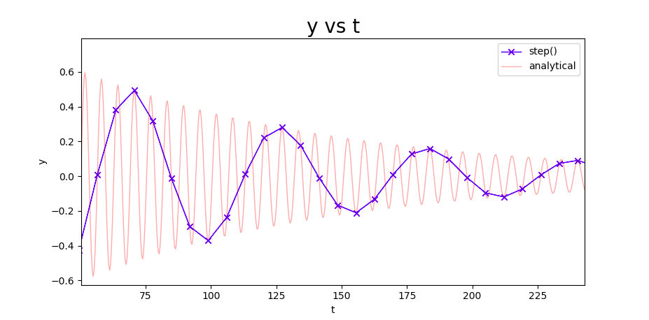
Somehow all cases like this seem to be using a fixed 100 time steps, instead of using more to avoid aliasing.
Scipy output is also identical - does the step function use scipy lti.signal.step?The code at https://github.com/ilayn/harold/blob/master/harold/_time_domain.py#L280-L454 mentioned in #287 works very well for this case with a good dt of 0.25 and ~1800 steps.
Thanks for pointing out the Harold code, @prashant2. I'm going to spend some time trying to fix up this problem as part of PR #383.
This is what I get from the current master of
harold.Gp = harold.Transfer(6,[1,6,11,6]) Gc = 10 Gor = Gp*Gc/(1 + Gp*Gc) # should have used feedback() command here anyways harold.step_response_plot(Gor)
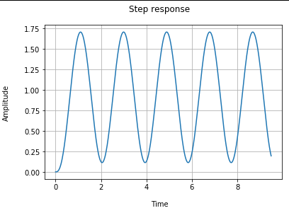
and for the other example
 a = -0.01
G1 = harold.Transfer([1,0],[1,-2*a, 1+a**2])
step_response_plot(G1)
Note that the dynamics are still decaying until 400s so I think Octave doesn't take that into account (in case you haven't specifically zoomed in).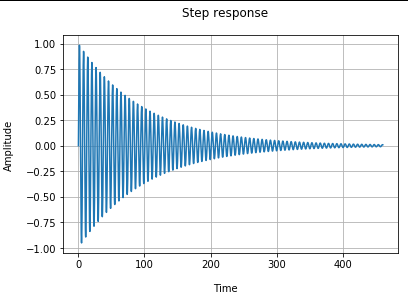
If this corona WFH thing lets me do some open source work, I'll try to release 1.0.2 soon. Please let me know if you encounter some nonsensical results.
Richard it would be great if you can look into the repeated pole sensitivity issue. The rest you can copy/paste at will if the code is useful (I can delicense it if needed no attribution etc. required).
- linked a pull request that will close this issueimproved default time vector for time response functions that takes zeros into account. #454
on Aug 19, 2020


I am trying to plot step response of a 3rd order process Gp, controlled with a P controller.
Gp = 6/[(s+1)(s+2)(s+3)]
I am using v0.8.3
Gor has 3 poles at (-6, sqrt(11) j, - sqrt(11) j ) and the expected behavior is sinusoidal oscillations after the initial transients have died down (ie t > ~ 2/3)
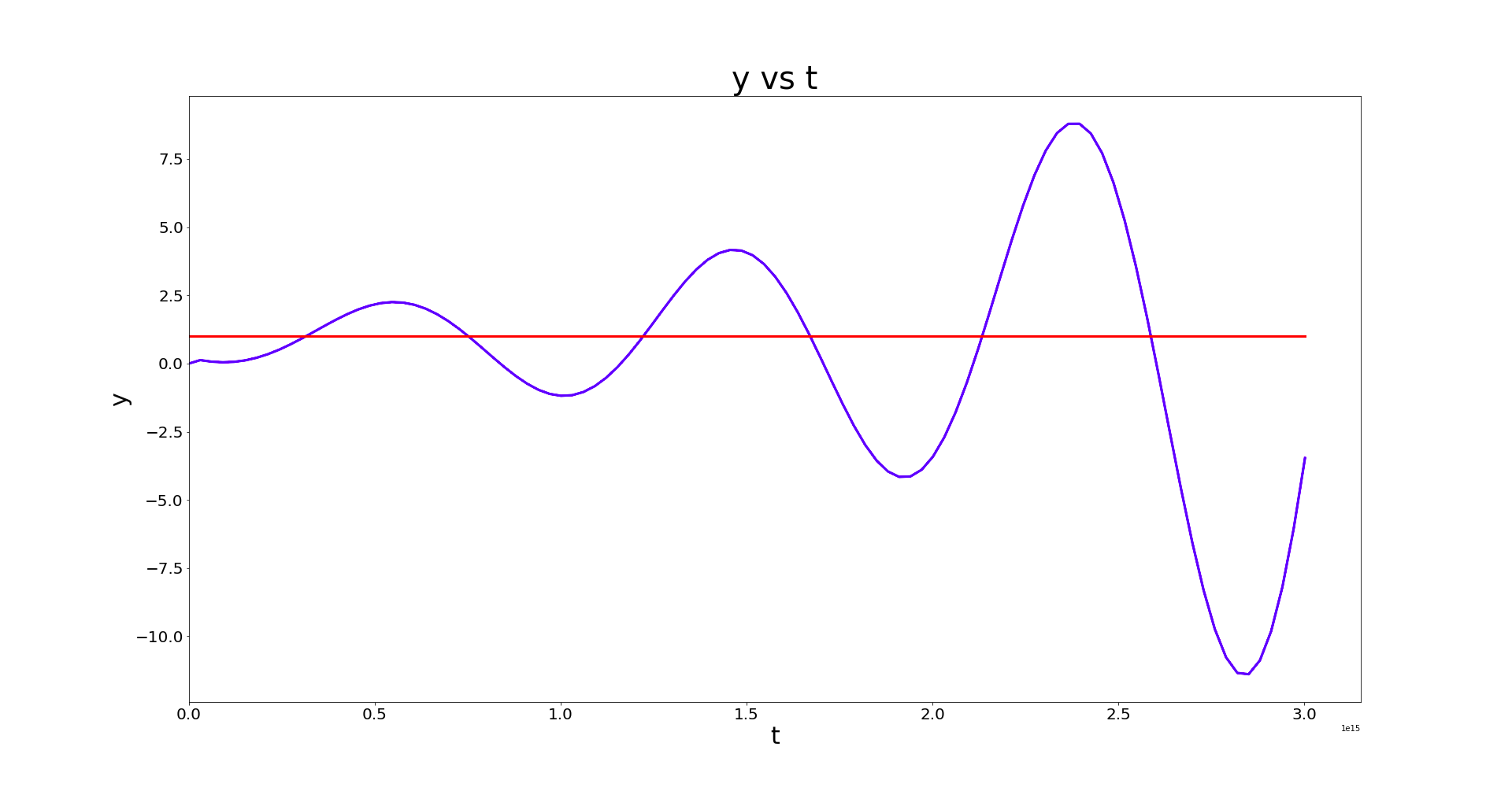
But what I get is an unstable system:
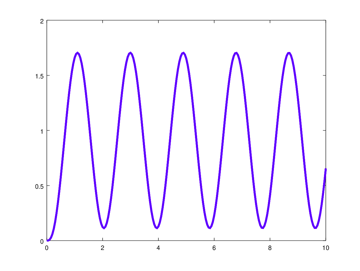
Octave gives the correct result (ymin 0.113, ymax 1.705 after transients):