Repository navigation
stability_margins doesn't find gain=1 crossover frequency correctly for DT systems #523

Description
Activity
why H(z)*H(1/z)=1 implies |H(z)| = 1
If I am not mistaken, it follows from
|H(z)|² = H(z) * conj(H(z)) = 1. Octave uses the same formulaBut the algorithm had a bug. Thanks for noticing and reporting.
- linked a pull request that will close this issuefix #523: finding z for |H(z)|=1 computed the wrong polynomials #525
on Jan 30, 2021 I see, Makes sense if we are restricting the root search to the unit circle, where 1/z = conj(z).
And it has been a little while but I guess it must be that h(conj(z)) = conj(h(z))
- added a commit that references this issue
on Jan 30, 2021 Reopening I found another example that seems to confuse the current version: a 4th order system consisting of two slightly-damped resonances in series:
import control as ct
omegan = 1
zeta = 0.5
resonance = ct.tf(omegan**2, [1, 2*zeta*omegan, omegan**2])
omegan2 = 100
resonance2 = ct.tf(omegan2**2, [1, 2*zeta*omegan2, omegan2**2])
sys = 5 * resonance * resonance2
#100*ct.tf(1,[1, 0]) * ct.tf([1, 1], [1, 100]) * resonance
sysd = ct.c2d(sys, .001)
This seems to give a reasonable result for the continuous-time case:
ct.bode_plot(sys, margins=True);
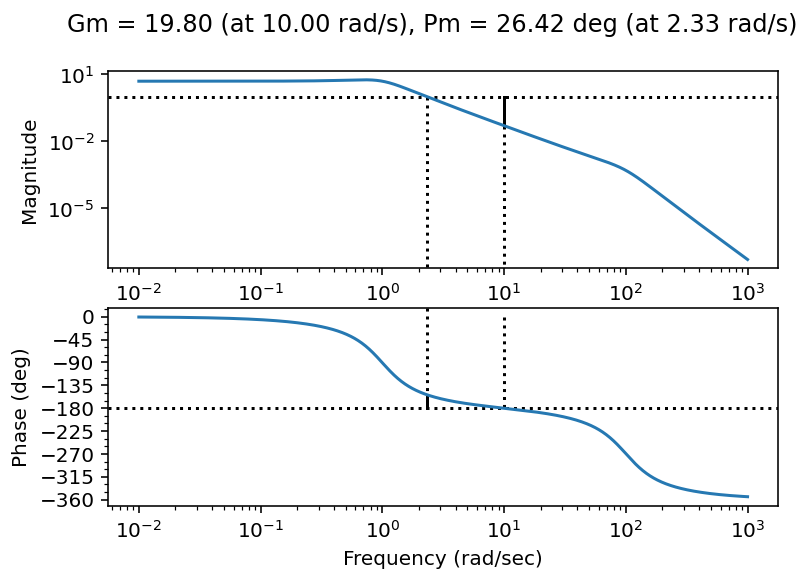
but not for the discrete-time case:
ct.bode_plot(sysd, margins=True);
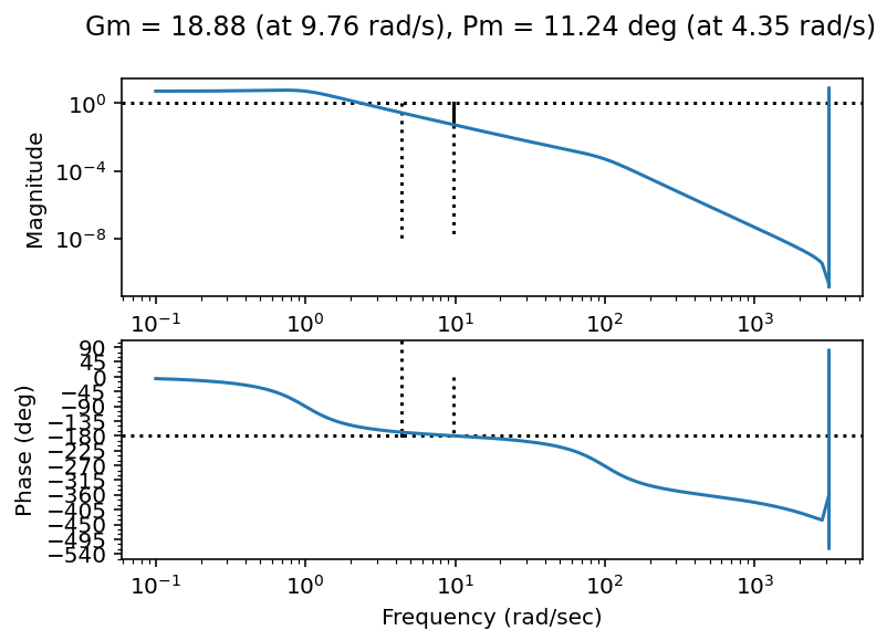
If I lower the damping ratio to
zeta=0.05it seems to be manage:
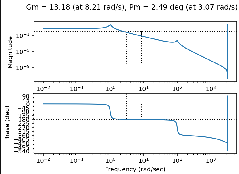
@bnagivator any ideas? I tried relaxing the tolerance but that didn't seem to help.
Numerical issues. The coefficients of the numerator are significantly smaller than those of the denominator.
python-control/control/margins.py
Lines 159 to 172 in 92de12d
IPdb [1]: num
array([2.04126716e-09, 2.19977183e-08, 2.15576756e-08, 1.92123173e-09])

IPdb [2]: den
array([ 1.        , -3.89432859,  5.69259981, -3.70220425,  0.90393303])

IPdb [3]: p1
array([3.92174723e-18, 8.62676896e-17, 5.60540187e-16, 9.56490893e-16,
       5.60540187e-16, 8.62676896e-17, 3.92174723e-18, 0.00000000e+00])

IPdb [4]: p2
array([  0.90393303,  -7.2224165 ,  25.25592868, -50.48489472,
        63.09489902, -50.48489472,  25.25592868,  -7.2224165 ,
         0.90393303])

IPdb [5]: np.polysub(p1, p2)
array([ -0.90393303,   7.2224165 , -25.25592868,  50.48489472,
       -63.09489902,  50.48489472, -25.25592868,   7.2224165 ,
        -0.90393303])

IPdb [6]: np.roots(np.polysub(p1, p2))
array([1.04733131+0.09092897j, 1.04733131-0.09092897j,
       0.94766452+0.08227594j, 0.94766452-0.08227594j,
       1.00290822+0.j        , 0.99999917+0.00307635j,
       0.99999917-0.00307635j, 0.99709245+0.j        ])

IPdb [7]: z
array([0.99999917+0.00307635j])

IPdb [8]: w
array([3.07634228])
The result of
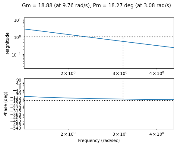
num(z)*num(1/z) - den(z)*den(1/z)is barely affected by the numerator, which gives an inaccurate result for the root. 😒My machine gives me a crossing frequency of 3.08 rad/s for
zeta=0.5too: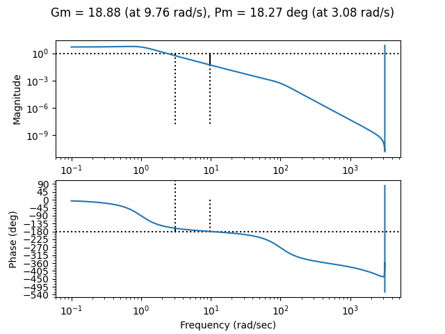
zoomed in:
I see. Looks like this may happen any time the nyquist frequency is maybe 3+ orders of magnitude faster than the slowest pole. What do you think about a stopgap solution to detect this by looking at the relative order of magnitudes of numerator and denominator polynomial and either give a warning or revert to the interpolating numerical solution via the FrequencyResponseData class?
I was thinking to use the inaccurate but not completely wrong found crossing frequency as a starting point for a local numerical solve. That way we don't have to evaluate the whole frequency range again.
Unfortunately I have another example where it is nowhere close (they invovle solutions to a class I am teaching so I will have to do some obfuscation before I can post them : )
Using an interpolating
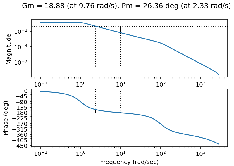
FrequencyResponseDatasystem as an intermediary produces pretty good results (see below). Which we could use as a starting point to get a better local numerical result using an optimizer as you suggested. What if I put in the FRD version as a stopgap (which will include some sort of a test for small numerator)? Yeah, it's slow. But it might serve as a starting point to do a better numerical solve?omega = ct.freqplot._default_frequency_range(sysd) sysdfrd = ct.FRD(sysd(np.exp(1j*sysd.dt*omega)), omega, smooth=True) ct.bode_plot(sysdfrd, omega=sysfrd.omega, margins=True);
On option might be to include a
methodkeyword someplace that allows you to tune the behavior of the calculation. So if you specifymethod='FRD'then you get the behavior above. This could be a way to keep from forcing every usage to be some slow method.(am hoping to have something working in place for 0.9 for the discrete-time controls class I'm teaching starting March 29. The students will appreciate a working DT margin calculation! : )
Reacted by Ben GreinerIf we can get this sorted out before ~22 March, we can do a 0.9.0 release that week to make it easy for students to install.
Reacted by Sawyer Fuller and Ben Greiner@murrayrm sure, a method keyword would make sense. What if I let that override things, but by default revert to the FRD method if it looks like the "old" method isn't going to give good numerical results?
Seems fine by me to have the default be something that works well.
You might consider setting up a benchmark file (in
benchmarks/) that lets you see how much of a performance hit there is on some different examples.In any case there should be a check, whether the current results are accurate enough and give a warning if not.
Reacted by Sawyer Fuller- linked a pull request that will close this issuenew method keyword in stability_margins and auto-fallback back to FRD .. #566
on Mar 13, 2021


stability_margins doesn't find gain=1 crossover frequency correctly for DT systems, but it seems to mostly do so for CT systems. I think the probelm may be in how
margins.poly_z_mag1_crossingis finding roots, but there were a few steps in that function I couldn't follow, e.g. why H(z)*H(1/z)=1 implies |H(z)| = 1.Example:
As an example of what it should look like, here is Matlab: