Repository navigation
frequency_response() returns incorrect response #860
Description
Activity
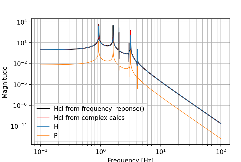
The frequency response is wrong due to numerical problems with the transfer function form. Transfer function form isn't good for high order systems, say order 10 or more. I can get the right result using state-space form, but it isn't quite as easy to construct the feedback loop as with TF form, since StateSpace doesn't support division.
Your feedback arrangement is unusual, but I've taken it at face value. The
minrealcalls aren't necessary, but made a difference when I had the wrong feedback form (feedback(H, P)instead ofH * feedback(1, P)).import numpy as np import matplotlib.pyplot as plt import pandas as pd import control # Importing State-Space matrices and check if dimensions are correct ssAspoiler = np.loadtxt(open('ssA_spoiler.csv', 'rb'), delimiter=',') ssB = np.loadtxt(open('ssB.csv', 'rb'), delimiter=',') ssC = np.loadtxt(open('ssC.csv', 'rb'), delimiter=',') ssD = np.loadtxt(open('ssD.csv', 'rb'), delimiter=',') print('dim(A) =', np.shape(ssAspoiler)) print('dim(B) =', np.shape(ssB)) print('dim(C) =', np.shape(ssC)) print('dim(D) =', np.shape(ssD)) # Define Frequency Array Frequency_Array = np.linspace(0.1, 100, int(1e5)) Omega_Array = Frequency_Array * (2*np.pi) # Create State-Space System sys = control.StateSpace(ssAspoiler, ssB, ssC, ssD) # Choose in- and outputs i1 = 0 i2 = 6 o = 12 # Extract TFs from State-Space System H = control.minreal(sys[o,i1]) P = control.minreal(sys[o,i2]) # Calculating (closed loop) TF from existing TF's # Feedback form inferred from Hcl = H/(1+P = H * (1 / (1+P) = H * feedback(1,P) Hcl = control.minreal(H * control.feedback(1, P)) # Compute frequency_response() of all TF from above mag_H, phase_H, _ = control.frequency_response(H, Omega_Array) mag_P, phase_P, _ = control.frequency_response(P, Omega_Array) mag_Hcl, phase_Hcl, _ = control.frequency_response(Hcl, Omega_Array) # Try different way to get proper frequency response of Hcl P_comp = mag_P * np.exp(1j*phase_P) H_comp = mag_H * np.exp(1j*phase_H) Hcl_comp = (H_comp) / (1 + P_comp) # Plot frequency responses plt.figure(dpi = 150, figsize = (10, 6)) plt.loglog(Frequency_Array, mag_Hcl, color = 'k', label = 'Hcl from frequency_reponse()') plt.loglog(Frequency_Array, np.abs(Hcl_comp), linewidth = .75, color = 'r', label = 'Hcl from complex calcs') plt.loglog(Frequency_Array, mag_H, label = 'H', linewidth = .75) plt.loglog(Frequency_Array, mag_P, label = 'P', linewidth = .75) plt.grid(True, which = 'both') plt.xlabel('Frequency [Hz]') plt.ylabel('Magnitude') plt.legend(loc = 'lower left') plt.show()
- locked and limited conversation to collaborators
on Mar 26, 2023


Hey,
I'm currently running version 0.9.2 and face some issues with the frequency_response() function with rather complex TransferFunctions. In my minimal working example, I create a MIMO system from state-space matrices with 24 in- and 18 outputs. In the next step, I extracted two transfer functions (H&P) and performed a simple calculation with both to create a new TF (Hcl). Using frequency_response() function on both the original TFs I get the expected result. For the new TF Hcl however, the response looks very messy in magnitude as well as in phase.
To get a short time fix, I took the frequency response of the original functions, converted magnitude and phase into a complex number and redid the calculation, which returned a the expected form of Hcl, as seen in the plot below.
The code i used is the following:
Since I want to use control.feedback() later on as well, this problem is especially problematic, since it also appears there.
Unfortunately, I can't pinpoint where this problem originates from, so I am hoping you might understand the reasons behind that. For completeness, I also attached the .txt files with the state-space matrices.
EDIT: I should mention, that I don't see this kind of behaviour for simple transfer functions.
ssD.csv
ssC.csv
ssB.csv
ssA_spoiler.csv