Repository navigation
Step Response and step_info accuracy issue #440

Description
Activity
- changed the title
[-]Step Response and step[/-][+]Step Response and step_info accuracy issue[/+]on Jul 29, 2020 The only "inaccuracy" here is the resolution of the time vectors
t1, t2:with python-control 0.8.3:
Python 3.8.3 (default, May 17 2020, 14:48:56) [GCC] on linux
Type "help", "copyright", "credits" or "license" for more information.
>>> from matplotlib import pyplot as plt
>>> import numpy as np
>>>
>>> import control
>>>
>>> print(control.__version__)
0.8.3
>>> num1 = [1.067e+05, 5.791e+04]
>>> den1 = [10.67, 1.067e+05, 5.791e+04]
>>> num2 = [1.881e+06]
>>> den2 = [188.1, 1.881e+06]
>>> sys_1 = control.TransferFunction(num1, den1)
>>> sys_2 = control.TransferFunction(num2, den2)
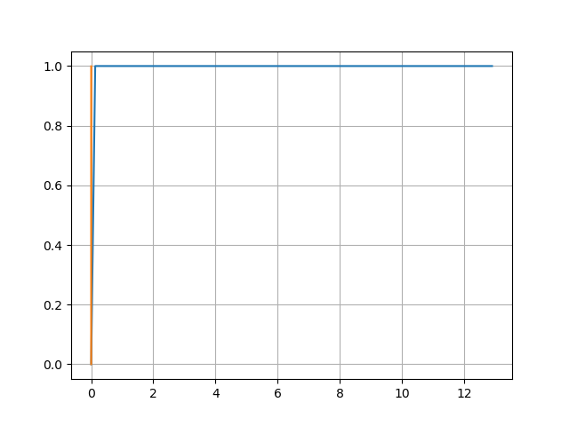
>>> t1, y1 = control.step_response(sys_1)
>>> t2, y2 = control.step_response(sys_2)
>>> print(control.step_info(sys_1))
{'RiseTime': 0.0, 'SettlingTime': 0.012909809495208709, 'SettlingMin': 1.0000000494992993, 'SettlingMax': 1.0000539034745675, 'Overshoot': 0.005385397260240271, 'Undershoot': 0.0, 'Peak': 1.0000539034745675, 'PeakTime': 0.012909809495208709, 'SteadyStateValue': 1.0000000494992993}
>>> print(control.step_info(sys_2))
{'RiseTime': 0.0002186186186186186, 'SettlingTime': 0.0003874874874874875, 'SettlingMin': 0.899570400385632, 'SettlingMax': 0.9990881180344406, 'Overshoot': 0.0, 'Undershoot': 0.0, 'Peak': 0.9990881180344406, 'PeakTime': 0.0007, 'SteadyStateValue': 0.9990881180344406}
>>> plt.plot(t1, y1, t2, y2)
[<matplotlib.lines.Line2D object at 0x7fa3bff24a30>, <matplotlib.lines.Line2D object at 0x7fa3bff24b20>]
>>> plt.grid()
>>> plt.show()
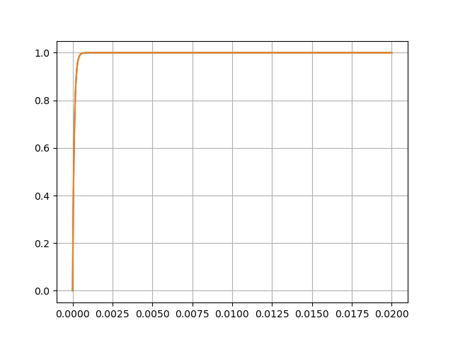
>>> T = np.linspace(0., 0.02, 1000)
>>> t1, y1 = control.step_response(sys_1, T=T)
>>> t2, y2 = control.step_response(sys_2, T=T)
>>> print(control.step_info(sys_1, T=T))
{'RiseTime': 0.0002202202202202202, 'SettlingTime': 0.0004004004004004004, 'SettlingMin': 0.9095372868757307, 'SettlingMax': 1.0000542217105208, 'Overshoot': 5.252466677250307e-05, 'Undershoot': 0.0, 'Peak': 1.0000542217105208, 'PeakTime': 0.001961961961961962, 'SteadyStateValue': 1.0000536964356492}
>>> print(control.step_info(sys_2, T=T))
{'RiseTime': 0.0002202202202202202, 'SettlingTime': 0.0004004004004004004, 'SettlingMin': 0.909499726158002, 'SettlingMax': 1.0000000000000002, 'Overshoot': 0.0, 'Undershoot': 0.0, 'Peak': 1.0000000000000002, 'PeakTime': 0.0035235235235235233, 'SteadyStateValue': 1.0000000000000002}
>>> plt.plot(t1, y1, t2, y2)
[<matplotlib.lines.Line2D object at 0x7fa3b44ea460>, <matplotlib.lines.Line2D object at 0x7fa3b44ea490>]
>>> plt.grid()
>>> plt.show()
Even with current master branch, which has #420 merged:
>>> from matplotlib import pyplot as plt
>>> import numpy as np
>>> import control
>>> print(control.__version__)
dev
>>> num1 = [1.067e+05, 5.791e+04]
>>> den1 = [10.67, 1.067e+05, 5.791e+04]
>>> num2 = [1.881e+06]
>>> den2 = [188.1, 1.881e+06]
>>> sys_1 = control.TransferFunction(num1, den1)
>>> sys_2 = control.TransferFunction(num2, den2)
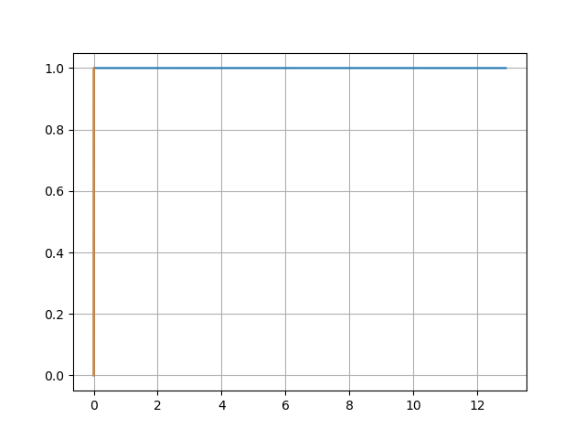
>>> t1, y1 = control.step_response(sys_1)
>>> t2, y2 = control.step_response(sys_2)
>>> print(control.step_info(sys_1))
{'RiseTime': 0.0, 'SettlingTime': 0.0025793799371427, 'SettlingMin': 1.000000049568649, 'SettlingMax': 1.0000542065543498, 'Overshoot': 0.0054156983016393195, 'Undershoot': 0.0, 'Peak': 1.0000542065543498, 'PeakTime': 0.0025793799371427, 'SteadyStateValue': 1.000000049568649}
>>> print(control.step_info(sys_2))
{'RiseTime': 0.00021700000000000002, 'SettlingTime': 0.000392, 'SettlingMin': 0.9007387484403545, 'SettlingMax': 0.9990219991316046, 'Overshoot': 0.0, 'Undershoot': 0.0, 'Peak': 0.9990219991316046, 'PeakTime': 0.000693, 'SteadyStateValue': 0.9990219991316046}
>>> plt.plot(t1, y1, t2, y2)
[<matplotlib.lines.Line2D object at 0x7fc593e92820>, <matplotlib.lines.Line2D object at 0x7fc593e92910>]
>>> plt.grid()
>>> plt.show()
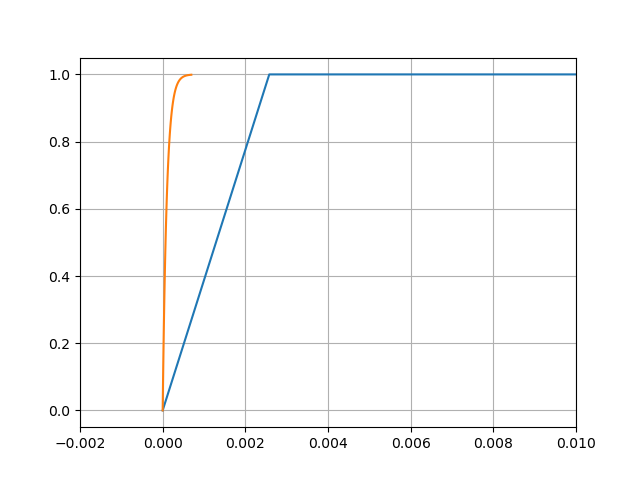
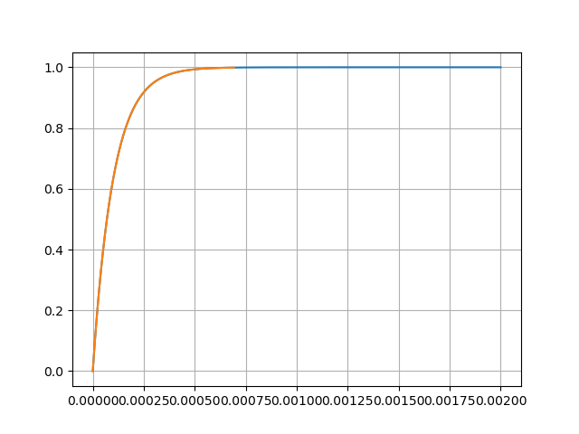
The magnitude of the canceling pole in
sys1still prevents the return of a good default time vector.>>> T = np.linspace(0., 0.002, 1000) >>> t1, y1 = control.step_response(sys_1, T=T) >>> plt.plot(t1, y1, t2, y2) >>> plt.grid() >>> plt.show()
 Reacted by Rajab Legnain
Thanks bnavigator,
Any plans to solve this? people coming form Matlab love to see similar results as in Matlab.
Flagging this for @sawyerbfuller to have a look since he wrote the current default response time calculation.
Reacted by Rajab LegnainHi @rlegnain indeed the current version of
step_responsechooses the time resolution of the step response based only on the poles and not the zeros. In particular, pole-zero cancellations will give it troubles. I wrote an update that is now in the development branch of the library that has an improved way of calculating the time vector, but it does not solve this problem.@ilayn was working on a solution that takes zeros into account in #287, and he posted his code here https://github.com/ilayn/harold/blob/master/harold/_time_domain.py#L280-L454, but I don't know how close he got to having a robust solution.
Reacted by Rajab LegnainI've tested for the given systems and indeed the responses are the same. The only remaining issue is when a system has Jordan blocks of significant poles but I think that is an open problem in the literature too. So with some reservation I would say it is robust but not fail-proof for every system.
Since we don't have the commercial ODE solvers I think that would be all we can do for now via utilizing only pole-zero information.
Reacted by Rajab LegnainThanks all.
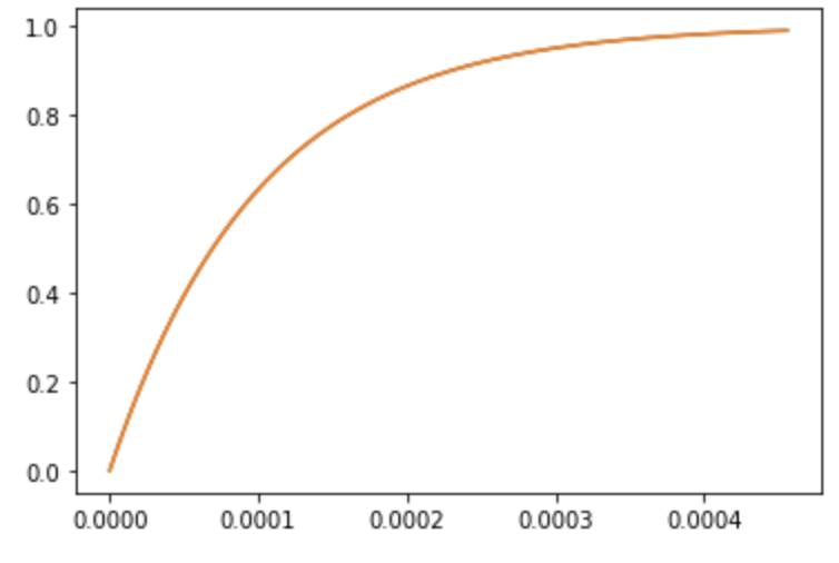
PR #454 , which incorporates @ilayn's code seems to fix this (both step responses are perfectly overlaid):
code output:
{'RiseTime': 0.0002118493270188449, 'SettlingTime': 0.0003500119315963524, 'SettlingMin': 0.8953357369737194, 'SettlingMax': 0.9895824151834175, 'Overshoot': 0.0, 'Undershoot': 0.0, 'Peak': 0.9895824151834175, 'PeakTime': 0.0004559365951057749, 'SteadyStateValue': 0.9895824151834175} {'RiseTime': 0.00021183782855545226, 'SettlingTime': 0.000349992934135095, 'SettlingMin': 0.8952871451949131, 'SettlingMax': 0.9895287145194958, 'Overshoot': 0.0, 'Undershoot': 0.0, 'Peak': 0.9895287145194958, 'PeakTime': 0.0004559118484128211, 'SteadyStateValue': 0.9895287145194958}Reacted by Rajab Legnain- linked a pull request that will close this issueimproved default time vector for time response functions that takes zeros into account. #454
on Aug 19, 2020


Hi,
I found an accuracy issue related to control.step_response and control.step_info. To be specific, the issue is in _default_response_times() function.
I have two system transfer function sys1 and sys2.They both have exactly the same frequency response.
sys1:
num1 = [1.067e+05, 5.791e+04], den1 = [10.67, 1.067e+05, 5.791e+04]
OR
k = 10000, zeros = [-0.5426], poles = [-1e+04, -0.5426 ]
sys2:
num2 = [1.881e+06], den2 = [188.1, 1.881e+06]
OR
k = 10000, zeros = [], poles = [-1e+04, ]
As you notice, sys1 has extra pole and zero where both have the same value.
The issue
When I plot the step responses for both systems, the plots are not matched. Also when I used step_info() to get the characteristics of the systems, I got a different results.
The code:
here is the code
Test on Matlab;
I tested the two systems in Matlab. The step() function gives the same step response plot for both systems, and stepinfo() results exactly the same values for both systems.