


Abstract
Future ocean acidification mainly depends on the continuous ocean uptake of CO2 from the atmosphere. The trajectory of future atmospheric CO2 is prescribed in traditional climate projections with Earth system models, leading to a small model spread and apparently low uncertainties for projected acidification, but a large spread in global warming. However, climate policies such as the Paris Agreement define climate targets in terms of global warming levels and as traditional simulations do not converge to a given warming level, they cannot be used to assess uncertainties in projected acidification. Here, we perform climate simulations that converge to given temperature levels using the Adaptive Emission Reduction Algorithm (AERA) with the Earth system model Bern3D-LPX at different setups with different Transient Climate Response to cumulative carbon Emissions (TCRE) and choices between reductions in CO2 and non-CO2 forcing agents. With these simulations, we demonstrate that uncertainties in surface ocean acidification are an order of magnitude larger than the usually reported inter-model uncertainties from simulations with prescribed atmospheric CO2. Uncertainties in acidification at a given stabilized temperature are dominated by TCRE and the choice of emission reductions of non-CO2 greenhouse gases (GHGs). High TCRE and relatively low reductions of non-CO2 GHGs, for example, necessitate relatively strong reductions in CO2 emissions and lead to relatively little ocean acidification at a given temperature level. The results suggest that choices between reducing emissions of CO2 versus non-CO2 agents should consider the economic costs and ecosystem damage of ocean acidification.

Original content from this work may be used under the terms of the Creative Commons Attribution 4.0 license. Any further distribution of this work must maintain attribution to the author(s) and the title of the work, journal citation and DOI.
1. Introduction
The Paris Agreement aims at limiting global warming well below 2 °C and at pursuing efforts to reduce warming to 1.5 °C to significantly reduce the risks and impacts of climate change [1]. To stabilize temperatures, the sum of CO2 forcing equivalent (CO2-fe) emissions [2, 3] from all greenhouse gases (GHGs) together must be close to net-zero [4–7]. The remaining allowable emissions of CO2 and non-CO2 forcing agents that can be emitted before net-zero must be reached depends among others on the Transient Climate Response to Cumulative Emissions (TCRE), i.e. the amount of warming per amount of cumulative emissions. TCRE depends on the transient climate response (or Equilibrium Climate Sensitivity (ECS)) and the strength of the ocean and land carbon sinks [2, 5, 8–16]. These allowable emissions can be distributed over all GHGs in many combinations. If relatively strong reductions in non-CO2 GHG emissions would be implemented, for example, the remaining allowable CO2 emissions will be relatively higher.
Globally averaged atmospheric surface warming is the main and often only measure of success or failure of the Paris Agreement, although climate impacts and stressors of ecosystems do not only or sometimes not at all depend on the level of global warming [17–19]. One example of such a potential ecosystem stressor is ocean acidification, a process that describes the gradual decrease in ocean pH, carbonate ions, and calcium carbonate mineral saturation states (Ω) in the ocean, which affects a variety of individual calcifying marine organisms and has the potential to disrupt entire ecosystems [20–30].
Future ocean acidification depends mainly on CO2 emissions and the perturbation in atmospheric and oceanic carbon cycle and is only marginally affected by the degree of warming [31], except in the Arctic Ocean [31, 32]. In surface waters, equilibrating rapidly with the atmosphere, acidification is primarily driven by atmospheric CO2 [23, 24, 33], with a regional role for alkalinity changes, e.g. in estuaries and the Arctic Ocean [34–38]. Acidification at depth depends mainly on how much of the anthropogenic carbon perturbation at the surface is transported to the deeper ocean [39–43].
As trajectories of future atmospheric CO2 are prescribed in the simulations from the Coupled Model Intercomparison Project (CMIP) by the socio-economic pathways [44, 45] that are used by the regular IPCC reports [46, 47], projections of ocean acidification have usually very low to non-existent model uncertainties at the ocean surface [18, 19, 33, 37, 48]. Therefore, these simulations cannot directly be used to inform policy makers about the uncertainties in ocean acidification and might, in the worst case, lead to overly confident projections on ocean acidification used for impact assessments. Only few studies assess uncertainties in projected ocean acidification comprehensively with prescribed carbon emissions by using perturbed parameter ensembles in simulations or by quantifying uncertainties as a function of cumulative carbon emissions [17, 49, 50]. These studies quantify uncertainties related to the land and ocean carbon sink but neither quantify uncertainties from the choice of GHG reductions (CO2 vs non-CO2) nor from the transient climate response to emissions. Such studies that quantify global ocean acidification and related uncertainties at a given level of global warming for different choices of GHG emission reductions remain missing.
The magnitude of ocean acidification and the associated uncertainty at a given stabilized temperature level can, however, be determined by simulations that adapt GHG emissions successively to converge to the same stabilized warming level. Such simulations prescribe the future warming level and not the atmospheric CO2 trajectories and hence do not quantify the uncertainty of warming per increase of atmospheric CO2 but the uncertainty of increases of atmospheric CO2 per warming. Approaches like the adjusting mitigation pathway (AMP) approach [51, 52] or the recently developed Adaptive Emission Reduction Approach (AERA) [53] allow to make such simulations with Earth system models by developing dynamically emission curves, which stabilize the simulated warming at any chosen temperature target. Here, we use the AERA, which accounts for all radiative agents and not only for CO2 as the AMP, in combination with a reduced-form atmospheric chemistry model and the Earth system model of Intermediate Complexity Bern3D-LPX with varying climate sensitives and ocean mixing rates [54, 55] to quantify ocean acidification when warming stabilized at 1.5 °C, 2.0 °C, 2.5 °C, and 3.0 °C above preindustrial temperature and the uncertainty due to varying TCREs, and the choice of reductions in CO2 and non-CO2 GHG emission. We use different configurations of Bern3D-LPX as a surrogate for a typical CMIP ensemble of Earth System Models (ESMs). The wide range of simulations with the AERA demonstrates that the main uncertainty of ocean acidification projection for a given warming stems mainly from the uncertainty in the knowledge of TCRE and the choice in the reductions in non-CO2 emissions. Moreover, the AERA simulations with Bern3D-LPX underline the importance of emission-driven temperature stabilization simulations in the CMIP framework for projections and uncertainty assessments of the Earth system, its carbon cycle [56], extreme events [43, 57], and ecosystem stressors [19] in a stabilized climate.
2. Methods
2.1. Adaptive emission reduction approach (AERA)
The AERA estimates a future trajectory of CO2-fe emissions [2, 3, 10] that allows to stabilize the global atmospheric surface warming at a prescribed temperature level in three steps solely based on past annually averaged trajectories of (a) CO2 emissions, (b) atmospheric CO2, (c) the radiative forcing of all non-CO2 forcing agents, and (d) global mean surface temperatures [53].
First, the AERA estimates the anthropogenic warming from the time series of radiative forcing and temperatures [58] using an impulse response function [59]. Second, the determined anthropogenic warming and the cumulative CO2-fe emissions (sum of CO2 emissions from fossil fuels and land use change and CO2-fe from non-CO2 radiative agents [3]) are used to determine the transient climate response to cumulative CO2-fe emissions (TCRE) [2, 3, 5, 8]. The TCRE then allows to estimate the remaining allowable emission budget (REB) of CO2-fe before the chosen temperature target is reached. In the third step, the CO2-fe in the REB are distributed over the next decades so that an overshoot in temperature is tried to be avoided and that year-to-year changes in CO2-fe emission reductions remain as small as possible. A detailed explanation of the AERA is provided by Terhaar et al [53].
2.2. Bern3D-LPX
Bern-3D-LPX is an Earth system model of intermediate complexity that simulates dynamically the physics, chemistry, and biology of the land biosphere, the ocean, and sea ice, as well as their coupling to the atmosphere [60, 61]. The model is used at nine different setups that cover TCREs from 1.35 °C (EgC)−1 to 2.16 °C (EgC)−1, which resembles the CMIP6 TCRE range of 1.32 °C–2.30 °C (EgC)−1 [62] and the observation-constrained range of 1.3 °C–2.3 °C (EgC)−1 [50] (EgC = 1000 PgC = 1018 gC). The range of TCREs is obtained by combinations of three different ocean diapycnal mixing parameters (3 × 10⁻⁵, 2 × 10⁻⁵, 1 × 10⁻⁵ m2 s−1) and three different climate feedback parameters (−0.1, −0.5, −1.0 Wm−2 K−1) that account for feedbacks in the Earth system that are not explicitly or potentially not correctly simulated by Bern3D-LPX. These setups were chosen as their range of ECSs from 2.3 to 4.6 °C covers the 5%–95% likelihood range of the latest ECS assessment based on multiple lines of evidence [63] and because the ocean mixing parameters result in a circulation that represents observed distributions of CFCs, O2, or Δ14C [61, 64].
2.3. Simulations and non-CO2 radiative agents
The simulations with Bern3D-LPX start in 1765 and are until 2025 all prescribed with the same CO2 emissions, non-CO2 radiative forcing, and land use area change. CO2 emissions are from the Global Carbon Budget until 2020 [65] and develop from 2021 to 2025 proportionally to the national determined contributions (NDC) as quantified by the Climate Action Tracker [66]. Non-CO2 radiative forcing is based on the RCP database until 2000 [67–71] and from 2000 to 2025 on the most recent assessment from chapter 7 in the IPCC AR6 WG1 [72] report using SSP2-4.5 as an extension of the historical period after 2014 [44] to better reflect historic CH4 and N2O emissions over the last years. Land-use change is prescribed from 1850 to 2100 based on SSP1-2.6 [73] and associated emissions are dynamically calculated by Bern3D-LPX. SSP1-2.6 was chosen for land-use change as CMIP simulations following this scenario result in temperature are on average between 1.5 °C and 2.0 °C [47], the temperature targets that are closest to the aims of the Paris Agreement to limit warming well below 2 °C and to pursue efforts to reduce it to 1.5 °C [1]. Volcanic radiative forcing is based on the Ice-core Volcanic Index 2 [74, 75] until 2000 and zero afterwards.
From 2025 to 2300, the emissions of CO2, N2O, CH4, CO, NOx , and VOC as well as trajectories of other non-CO2 radiative agents, such as aerosols, evolve dynamically to match the prescribed CO2-fe emission curve, which is updated every five years. The AERA is first applied in 2025 and then every five years to mimic the stock take process foreseen in the Paris Agreement that includes a new submission of world-wide NDCs every five years with the next NDC submission being in 2025. The emissions of N2O, CH4, CO, NOx , and VOC are used by a reduced form atmospheric chemistry model to calculate their respective atmospheric concentrations and the associated radiative forcing and CO2-fe emissions. A detailed explanation of the reduced atmospheric chemistry model and parameters is provided by Terhaar et al [53]. The ozone forcing and the aerosol forcing in the atmospheric chemistry model was here changed to 0.47 Wm−2 and −1.06 Wm−2 in 2019, respectively, to match the non-CO2 radiative forcing from the IPCC AR6 WG1 report [72].
As many combinations of the different GHGs and radiative agents exist that would lead to the same prescribed CO2-fe emission curve, prior assumptions must be made for the evolution of the non-CO2 radiative agents. Three sets of simulations were made to represent a wide range of future choices (supplementary table 1). In the first set of simulations, called ‘baseline’, CH4 and N2O emissions evolve after 2020 according to SSP2-4.5, under which global warming will likely be limited to 2 °C warming [76], and CH4 and N2O emissions are constant from 2100 onwards (supplementary figure 1). Although SSP1-2.6 represents the scenario that results in temperatures closest to the Paris Agreement targets (see above), we chose SSP2-4.5 to provide a set of simulations were CO2 reductions are relatively higher so that the three sets of simulations span a range of CO2 emissions. In addition, the aerosol radiative forcing decreases exponentially (80% with a lifetime of 100 years, and 20% with a lifetime of 50 years). CO2 emissions evolve dynamically so that the total CO2-fe emission match the AERA-prescribed CO2-fe emissions. In the second set of simulations, called ‘high-CO2 ’, aerosols also decrease exponentially as in the ‘baseline’ simulations and CH4 and N2O emissions evolve parallel to CO2 emissions. The parallel evolution causes CH4 and N2O emissions to decrease faster than under SSP2-4.5 and result accordingly in smaller CO2-fe emissions from CH4 to N2O. Reductions in CO2 emissions can therefore be weaker to still equal the same CO2-fe emission than in the baseline simulation, which yields comparatively higher CO2 emissions. In the third set of simulation, called ‘constant aerosol’, CO2, CH4, and N2O emissions also evolve proportionally but the aerosol radiative forcing remains at 2025 levels. Therefore, even less stringent CO2 emission reductions are necessary in this set of simulations to reach the temperature targets and CO2 emissions and, in turn, atmospheric CO2 can remain higher than in the ‘baseline’ and ‘high-CO2’ simulations. Land-use change remains unchanged across all simulations.
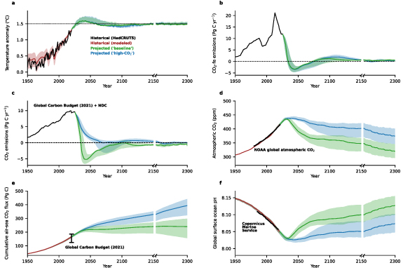
Figure 1. Temperature anomalies, associated CO2 forcing equivalent emissions, and carbon cycle dynamics. (a) Global mean surface temperature anomalies over the historical period until 2020 as observed by HadCRUT5 [82] (black line) and as simulated by the Bern3D-LPX (brown). After 2020, projections are shown for the 1.5 °C target for the ‘baseline’ (green) and high-CO2 (blue) scenarios. The dashed black line shows the 1.5 °C temperature target. (b) CO2 forcing equivalent (CO2-fe) emissions and (c) CO2 emissions as prescribed from the global carbon budget 2021 [65] and NDCs until 2025 (black) and adaptively developed by the AERA from 2025 onwards. The dashed lines represent zero emissions. Simulated (d) atmospheric CO2, (e) cumulative air-sea CO2 flux since 1765 (annual air-sea CO2 fluxes are shown in supplementary figure 2), and (f) globally averaged surface ocean pH. The green and blue lines indicate simulations with the model setup that has an ECS of 3.2 °C, the central estimate according to Sherwood et al [63]. The shading indicates the range of all model setups with ECS’ from 2.3 °C to 4.7 °C (5%–95% ECS likelihood range) [63]. In addition, observation-based estimates of the (d) past global atmospheric CO2 from NOAA averaged over marine surface sites [80], the (e) historical cumulative ocean carbon uptake from the global carbon budget 2021 [65], and the (f) past global surface average pH from the Copernicus Marine Service (https://doi.org/10.48670/moi-00047) is shown.
Download figure:
Standard image High-resolution imageThroughout the manuscript, we focus on the ‘baseline’ and ‘high-CO2’ simulations that rely only on emission reductions, which are the only sustainable to reach a prescribed temperature target [77]. As opposed to these mitigation scenarios, the ‘constant aerosol’ simulations also rely on strong aerosol injection via solar radiation modification to keep the aerosol forcing constant. Solar radiation modification is only an emergency solution as it comes with high risks, e.g. an abrupt rise in temperatures if the solar radiation modification should fail in the future for technical or political reasons [78], further commitments and unintended side effects like shifting monsoon patterns, changes in meridional temperature gradients, atmospheric and oceanic circulation, and the modes of climate variability [79]. By presenting solar radiation modification briefly in the main manuscript and more detailed in the Supplementary Material, we transparently show all theoretical options but focus on the sustainable and more likely options.
In all simulation, CH4 and N2O emissions have lower limits of 30 Tg CH4 yr−1 and 5.3 Tg N2O yr−1 due to non-abatable emissions in agriculture and livestock sectors. Simulations for the three set of simulations were made for four temperature targets of 1.5°C, 2.0 °C, 2.5 °C, and 3.0 °C with each of the nine setups of Bern3D-LPX representing ECS’ from 2.3 °C to 4.7 °C, resulting in 108 simulations (3 set of simulations ×4 temperature targets ×9 Bern3D-LPX setups). As Bern3D-LPX underestimates the inter-annual variability, each of these 108 setups was made with eight temporally varying superimposed inter-annual surface atmospheric temperature variabilities that are derived from observations [53] and hence yield 864 simulations in total (3 set of simulations ×4 temperature targets ×9 Bern3D-LPX setups ×8 temperature variabilities; supplementary table 1). The presented simulation results are openly available [83].
As all setups with different ECS simulate a different historical warming until 2020 compared to the 1850–1900 period (0.83 °C–1.39 °C), the remaining emissions and increases in atmospheric CO2 until a chosen temperature target is reached depends sensitively on this past warming. To remove this uncertainty, the temperature target is always defined relative to the observation-based anthropogenic warming in year 2020, which is estimated to be 1.23 ± 0.20 °C [53]. For the 1.5 °C target, this means that an allowable warming of 0.27 °C remains. This allowable warming is then added to the anthropogenic warming in each setup. This Δ-approach is the same that is regularly used for ocean acidification studies where different models have difficulties to simulate the baseline biogeochemistry in the interior ocean at present [23, 37, 39, 40].
3. The carbon cycle and ocean acidification in a stabilized 1.5 °C world
3.1. Uncertainty from the transient climate response to cumulative carbon emissions
The simulated historical temperature anomaly with respect to 1850–1900 under prescribed CO2 emissions increases at a similar pace as the observed temperature over all nine model setups (±0.25 °C), despite varying climate sensitivities and ocean carbon sink strengths (figure 1(a)). All model setups do not only capture the historical temperature trajectory, but also the observed trajectory of atmospheric CO2 [80] (figure 1(d)), the observation-based estimate of the cumulative ocean carbon uptake [65] (figure 1(e)), and the globally averaged pH over the last decades (figure 1(f)).
After the AERA is switched on in 2025, all trajectories converge by 2150 within ±0.05 °C to the prescribed 1.5 °C temperature target because fossil fuel CO2 emissions evolve freely so that the combined CO2-fe emissions from fossil fuels, land use change, and non-CO2 radiative agents match the prescribed CO2-fe emissions by the AERA. The total CO2-fe emissions from 2021 to 2150 that allow to meet the 1.5° target vary from −59 Pg C to +203 Pg C (range of nine setups after averaging over all eight realizations with varying inter-annual superimposed variability) under the ‘baseline’ scenario (figure 1(b)). The uncertainty ranges (−35 Pg C to +239 Pg C under the ‘high-CO2’ scenario; −27 Pg C to +255 Pg C under the ‘constant aerosol’ scenario) differ between the three scenarios due to the good but imperfect transformation of non-CO2 radiative forcing to CO2-fe emissions. In simulations with the AERA that converge to a temperature target, the uncertainty from the TCRE transfers into the CO2-fe budget, whereas traditional projections used in the IPCC reports [47] based on shared socioeconomic pathways (SSPs) [44, 45, 81] have an inter-model temperature range for a given CO2-fe trajectory (for example, the 5%–95% range for global warming in 2100 under SSP1-2.6 is 1.3 °C–2.8 °C) [47].
The range of cumulative CO2-fe emissions from 2021 to 2150 that allow to meet the 1.5 °C target (−59 Pg C to +203 Pg C for the ‘baseline’ scenario) propagates directly into different fossil fuel CO2 emission trajectories. The remaining allowable fossil fuel CO2 emissions depend on AERA derived CO2-fe emissions and the non-CO2 emissions and the CO2 emissions from land-use change. In the ‘baseline’ scenario, CH4 and N2O emissions and aerosols follow prescribed trajectories, resulting in CO2-fe emissions of all non-CO2 radiative agents from 2021 to 2150 of 160 Pg C and land-use change emissions of 17 Pg C. Therefore, the remaining allowable fossil-fuel CO2 emissions from 2021 to 2150 under this scenario range from −236 Pg C to +25 Pg C (figure 1(c)).
The range of CO2 emission trajectories affects the projected atmospheric CO2 and the rates and magnitude of ocean carbon uptake (figures 1(d) and (e), supplementary figure S2). By 2150, possible atmospheric CO2 in a 1.5 °C world under the ‘baseline’ scenario range from 320 ppm to 368 ppm after having peaked at 433–439 ppm between 2030 and 2035, and the cumulative ocean carbon sink from 1765 to 2150 varies from 190 Pg C to 271 Pg C. In comparison, the SSPs that are used by the IPCC have by definition no uncertainty in the future atmospheric CO2 as atmospheric CO2 is prescribed as a boundary condition. While the uncertainty of the atmospheric CO2 in 2100 is by definition non-existent, the range of the cumulative carbon sink is also smaller when atmospheric CO2 is prescribed, for example 274–332 Pg C for SSP1-2.6 across the CMIP6 ensemble [56]. Thus, when CO2 emissions evolve freely to converge to a temperature target, the range of the future sink is ∼40% larger than under fixed atmospheric CO2.
The wide range of possible atmospheric CO2 translates into different surface ocean pH projections. At the ocean surface changes in pH are almost entirely driven by changing dissolved inorganic carbon [57], which in turn closely follows the changes in atmospheric CO2 due to the air-sea CO2 flux that tends to equilibrate differences in CO2 partial pressure between the atmosphere and ocean. Hence, the projected atmospheric CO2 range from 320 ppm to 368 ppm in 2150 results in an almost perfectly anti-correlated projected range in surface ocean pH from 8.079 to 8.129 (after a minimum of 8.024–8.033 between 2031 and 2037) (figures 1(d)–(f)). This range is an order of magnitude larger than the projected standard deviation in projected ocean surface pH of ±0.002 under SSP1-2.6 in 2100 [19]. Furthermore, the annually averaged surface area that is projected to have saturation states of aragonite—a mineral form of calcium carbonate produced by marine organisms—below one remains almost non-existent (<106 km2) due to the rapidly decreasing CO2 emissions. However, saturation states may still drop below one on diurnal [84, 85] or seasonal [31, 86] timescales or in the 126 m below the surface (figure 3(f), supplementary figure 3), where calcifying organisms vertically migrate [87].
As opposed to surface ocean acidification, long-term ocean acidification below the surface depends not only on the increasing surface ocean dissolved inorganic carbon but also on the quantity of additional dissolved inorganic carbon at the ocean surface that is transported below the ocean surface [31, 37, 39, 40, 56, 88] and distributed within the ocean [42, 89]. The decrease in the global ocean volume that is projected to remain saturated towards aragonite (ΩA > 1) from 2002 to 2150 ranges from 47 to 86 × 106 km3 (17%–32% of supersaturated volume in 2002) (figure 2(a)), with the central estimate (setup with ECS = 3.2 °C) being 71 × 106 km3 (26%) and the standard deviation across all nine setups being 12 × 106 km3 (4%). Similarly, the range in volumes changes with ΩA between 1 and 2, 2 and 3, and above 3 vary strongly across the different model setups. Under prescribed atmospheric CO2 in SSP1-2.6, the simulated decrease in volume that is projected to remain saturated towards aragonite (ΩA > 1) in 2100 is 89 ± 6 × 10⁶ km3 [56]. Thus, the uncertainty of future interior ocean acidification rates under a prescribed temperature target when using the AERA is around twice as large as under prescribed atmospheric CO2. The difference in uncertainty under prescribed temperature targets and prescribed atmospheric CO2 is smaller in the ocean interior (factor 2) than at the ocean surface (factor 10), because most water masses are not in direct contact with the atmosphere so that the differences in simulated ocean circulation and deep-water formation affects both kinds of simulations [37, 39, 40, 56, 90, 91].
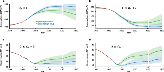
Figure 2. Interior ocean aragonite saturation state over time. Global mean ocean volume of water masses with aragonite saturation states (a) below 1, (b) between 1 and 2, (c) between 2 and 3, and (d) above 3 as simulated by the Bern3D-LPX until 2020 (brown) and from 2020 to 2300 for the 1.5 °C target under the ‘baseline’ (green) and ‘high-CO2’ (blue) scenario. The lines indicate simulations with the model setup that has an ECS of 3.2, the central estimate according to Sherwood et al [63]. The shading indicates the range of all model setups with ECSs from 2.3 °C to 4.7 °C (5%–95% ECS likelihood range [63]). Saturation states in 2002 are calculated from observation-based global ocean estimates of dissolved inorganic carbon, alkalinity, temperature, salinity, silicon, and phosphorus from GLODAPv2 [92]. For all other years, saturation states are calculated from the observation-based dissolved inorganic carbon, alkalinity, temperature, salinity, silicon, and phosphorus in 2002 plus the respective simulated changes in with respect to 2002 [23, 37, 40]. The same timeseries for the upper 126 m are shown in supplementary figure 3.
Download figure:
Standard image High-resolution image3.2. Uncertainty from the choice of reductions of non-CO2 radiative agents
The evolution of non-CO2 radiative forcing agents does not influence the temperature and CO2-fe trajectory (figures 1(a) and (b)) but limits, for a given temperature target, the range of possible future trajectories of CO2 emissions, atmospheric CO2, ocean carbon uptake, surface ocean pH, and interior ocean aragonite saturation states (figures 1(c)–(f) and 2). Under the ‘baseline’ scenario, non-CO2 radiative agents are prescribed following SSP2-4.5 and the radiative forcing of major non-CO2 radiative agents (N2O, CH4, and aerosols) under SSP2-4.5 do not get strongly reduced. Thus, the reduction in CO2-fe emissions as prescribed by the AERA is achieved via reductions in CO2 emissions. As opposed to the ‘baseline’ scenario, the radiative forcing or emissions of the major non-CO2 radiative agents are reduced strongly under the ‘high-CO2’ scenario so that CO2 emissions remain higher from 2025 to 2075, yielding a remaining CO2 budget from 2021 to 2150 of 54–286 Pg C, significantly larger than the −236 Pg C to +25 Pg C range under the ‘baseline’ scenario. As CO2 emissions are larger under the ‘high-CO2’ scenario, so are atmospheric CO2 (371–420 ppm in 2150 after having peaked at 436–445 ppm between 2034 and 2043), and the cumulative carbon uptake by the ocean (281–352 Pg C in 2150).
The larger atmospheric CO2 in the ‘high-CO2’ scenario and the larger cumulative carbon uptake by the ocean result in higher ocean acidification. The range of projected surface ocean pH across the nine different model setups with stronger reduction in non-CO2 radiative agents is 8.033–8.080 in 2150 (after a minimum of 8.018–8.029 between 2042 and 2047) (figures 1(d)–(f)). The decrease in volume that is projected to remain saturated towards aragonite (ΩA > 1) in 2150 under the ‘high-CO2’ scenario ranges from 86 to 111 × 106 km3 (31%–41%) (figure 2(a)). Overall, the choice of non-CO2 radiative forcing agents hence increases the possible range of ocean acidification rates in a 1.5 °C world by a factor of two and makes the uncertainty about the future ocean acidification rates in a 1.5 °C world thus even larger than it already was due to the different TCRE’s (see above). The entire range of globally averaged surface ocean pH under both scenarios of 0.096 is thus as large as the difference in surface ocean pH between SSP1-2.6 (warming of 1.3 °C–2.8 °C [47]) and SSP2-4.5 (warming of 2.1 °C–4.0 °C) and ∼50 times as large as the inter-model difference for each scenario across the range of CMIP6 Earth system models [19].
In addition to the ‘high-CO2’ scenario, the ‘constant aerosol’ scenario allows to assess a potential future in which the necessary GHG reductions are compensated by continuing aerosol emissions so that the cooling effect of aerosols in the atmosphere does not reduce over the 21st century. In that scenario, the CO2 emissions can remain even higher, yielding higher atmospheric CO2 in 2150 (411–465 ppm), higher ocean cumulative CO2 uptake from 1765 to 2150 (335–405 Pg C), and much more severe ocean acidification with globally averaged pH values in 2150 ranging from 7.998 to 8.045 (supplementary figure 4). This example demonstrates the importance of multiple climate targets [17] in addition to temperature targets to reduce the damaging effect of anthropogenic emissions on Earth ecosystems.
4. The carbon cycle and ocean acidification if global warming permanently exceeds the temperature targets of the Paris Agreements
The Paris Agreement aims at limiting global warming well below 2 °C and reducing it to 1.5 °C [1]. However, recent carbon and non-CO2 GHG emissions suggest that this target may not be met [66, 93]. Hence, it is important to quantify the effect of different warming levels that permanently overshoot the Paris Agreement temperature goals on the carbon cycle and ocean acidification. In this section, the projected atmospheric CO2, ocean carbon uptake, surface ocean pH, and interior ocean ΩA are quantified for a 2.0 °C, 2.5 °C, and 3.0 °C target (figure 3, supplementary table 2) although many other targets would be possible.
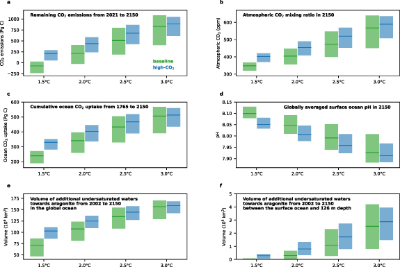
Figure 3. Projected carbon cycle and ocean acidification under various temperature targets. (a) Remaining CO2 emissions from 2021 to 2150 that allow meeting the temperature targets, (b) atmospheric CO2 in 2150, (c) cumulative ocean carbon uptake from 1765 to 2150, (d) globally averaged surface ocean pH in 2150, and (e) the additionally undersaturated waters towards aragonite from 2002 to 2150 for the ‘baseline’ (blue) and ‘high-CO2’ (blue) scenarios for stabilized warming at 1.5 °C, 2.0 °C, 2.5 °C, and 3.0 °C for the entire ocean and (f) only for the upper 126 m below the surface. The thick lines represent the model setups that has an ECS of 3.2 °C, the central estimate according to Sherwood et al [63]. The colored shading indicates the range across all nine setups. All results were averaged across the eight realizations of each setup with varying superimposed inter-annual variability.
Download figure:
Standard image High-resolution imageWith increasing warming, the range across setups increases as the transient climate response to cumulative emissions (TCRE) leads to a higher range in the remaining emission budget for a higher temperature target. In 2150, when the temperature stabilizes in these simulations, the higher range in the remaining emission results in large uncertainty ranges in past cumulative CO2 emissions and ocean carbon uptake, as well as large ranges in atmospheric CO2, surface ocean pH, and the volume of water undersaturated towards aragonite are simulated across the different model setups. These ranges even overlap for different temperature targets. Under the ‘baseline’ scenario, even the projections for the 2.0 °C and 3.0 °C target almost overlap. When adding uncertainties from the choice of the non-CO2 emissions, the projections of the 2.0 °C and 3.0 °C targets overlap strongly. Furthermore, the differences between the projections of the carbon cycle between the ‘baseline’ and ‘high-CO2’ are reduced under higher temperature targets because non-CO2 emissions under the ‘high-CO2’ are proportional to CO2 emissions. As CO2 emissions remain higher for a warmer temperature target so are the emissions of non-CO2 radiative agents, which remain hence closer to the prescribed emissions of non-CO2 radiative agents under the ‘baseline’ scenario.
Overall, the comparison demonstrates the large uncertainties of the carbon cycle projections under prescribed temperature targets, which are not apparent under usual projections by Earth system models under RCPs or SSPs with prescribed trajectories of atmospheric CO2 and non-CO2 radiative agents.
5. Conclusion
The simulations with the AERA allow assessing the so-far largely unknown uncertainties of the ocean carbon cycle and ocean acidification under prescribed temperature targets. Until now, future ocean acidification was assessed by the IPCC [33] and other studies [18, 19] using scenarios with prescribed atmospheric CO2 trajectories [18, 19, 33] and only few studies assessed uncertainties in acidification metrics by prescribing, adapting, or remapping carbon emissions [49–52]. The uncertainties for global and regional ocean acidification projections under prescribed atmospheric CO2 trajectories were reduced with great efforts by understanding differences between the different Earth system models [37, 39, 40, 56]. However, here we show that the uncertainties stemming from the TCRE, which is determined by the Earth’s warming response to GHGs, e.g. ECS, and ocean carbon uptake, are twice as large to a magnitude larger than the inter-model differences in the usual projections.
The here provided simulations are made with an Earth system model of intermediate complexity and provide robust projections of the globally or basin-wide averaged projections. For projections of ocean acidification on a regional scale like the Gulf of Alaska [94], the Eastern Boundary upwelling systems [95, 96], the Arctic Ocean [37, 40], or the Southern Ocean [39, 89], state-of-the-art Earth system models representing small scale circulation [42, 97–99] would need to be run with the AERA in the future.
The difference in the projected future of the ocean carbon uptake and ocean acidification also highlights the importance of the choice of emission reductions between CO2 and non-CO2 emissions for the ocean ecosystems that are vulnerable to ocean acidification. While many different combinations of reductions in CO2 and non-CO2 emissions allow reaching a given temperature target, these different combinations may affect ecosystems vulnerable to ocean acidification in very different ways. In the case of ocean acidification, the same amount of CO2-fe emissions in form of CO2 emissions is more harmful to the ocean than in form of N2O or CH4 emissions. Moreover, the possible implementation of solar radiation modification, e.g. via continuing aerosol emissions, to limit global warming to 1.5 °C would still cause high ocean acidification rates. Hence, when agreeing on climate targets policy makers should not only focus on warming levels [1], but also on other climate targets [17].
Acknowledgments
This work was funded by the European Union’s Horizon 2020 research and innovation program under Grant Agreement No. 821003 (Project 4C, Climate–Carbon Interactions in the Current Century) (Jens Terhaar, Thomas L Frölicher, Fortunat Joos) No. 820989 (Project COMFORT, Our common future ocean in the Earth system-quantifying coupled cycles of carbon, oxygen and nutrients for determining and achieving safe operating spaces with respect to tipping points) (Thomas L Frölicher, Fortunat Joos), and No. 101003687 (Project PROVIDE, Paris Agreement Overshooting) (Thomas L. Frölicher) as well as by Woods Hole Oceanographic Institution Postdoctoral Scholar Program (Jens Terhaar), and the Swiss National Science Foundation under Grant PP00P2_198897 (Thomas L Frölicher) and Grant #200020_200511 (Jens Terhaar, Fortunat Joos). This study has been conducted using E.U. Copernicus Marine Service Information; https://doi.org/10.48670/moi-00047. The work reflects only the authors’ view; the European Commission and their executive agency are not responsible for any use that may be made of the information the work contains.
Data availability statement
The data that support the findings of this study are openly available at the following URL/DOI: https://doi.org/10.17882/92735.
Author contributions
J T, T L F, and F J are responsible for conceptualization and methodology. J T made the simulations, analyses, visualization, and wrote the original draft. T L F and F J were responsible for funding acquisition. T L F and F J were responsible for project administration. J T, T L F, and F J were responsible for writing, review, and editing.
Conflict of interest
The contact author has declared that none of the authors has any competing interests.


