Image masks of global ship tracks for NASA MODIS data products

Abstract

Ship tracks, long thin artificial cloud features formed from the pollutants in ship exhaust, are satellite-observable examples of aerosol-cloud interactions (ACI) that can lead to increased cloud albedo and thus increased solar reflectivity, phenomena of interest in solar radiation management. In addition to ship tracks being of interest to meteorologists and policy makers, their observed cloud perturbations provide benchmark evidence of ACI that remain poorly captured by climate models. To broadly analyze the effects of ship tracks, high-resolution satellite imagery data highlighting their presence are required. To support this, we provide a hand labelled dataset to serve as a benchmark for a variety of subsequent analyses. Established from a previous dataset that identified ship track presence using NASA’s MODIS Aqua satellite imager, our first-of-its-kind dataset is comprised of image masks: capturing full ship track regions, including their contours, emission points and dispersive patterns. In total, 300 images, or around 2,500 masked ship tracks, observed under varying conditions are provided, and may facilitate training of machine learning algorithms to automate extraction.

Background & Summary

Satellite payloads that include geostationary sensors, frequently detect long thin artificially created ship tracks in boundary layer clouds above large oceanic regions. These features are a result of the high concentrations of cloud condensation nuclei (CCN) that form from the nitrogen and sulfur oxides present in ship exhaust. In other words, the pollutants in ship exhaust can seed low-lying marine clouds by enhancing cloud droplet formation. However, because the clouds are water vapor limited, even in the marine boundary layer, cloud droplets, albeit more numerous, are typically smaller in clouds that have been influenced by ship effluents¹. While suppression of droplet size may reduce the precipitation produced by marine clouds, the enhancement of droplet concentration from ship exhaust results in higher cloud albedo^2,3. The microphysical process through which ship exhaust modulates cloud reflectivity is similar to a proposed climate adaptation strategy known as Marine Cloud Brightening (MCB)⁴, which is actively being studied as a potential solar climate intervention mechanism to slow down the impact of global warming, by reflecting more solar radiation back to space^5,6,7,8,9. The study of ship tracks: satellite observable phenomena of natural MCB experiments, is thus critical in the development of MCB strategies.

The relatively bright tracks that may result from higher cloud albedos can persist for several hours after initial injection, before tracks fully disperse and become visibly indiscernible from other cloud features. However, it has been documented that a significant fraction of incoming solar energy reflected by tracks likely occurs over a longer lifetime (within 1-3 days after injection), with other studies indicating that clouds may take between a few hours to a few days to adjust and respond to aerosol injection⁵. In addition to determining the efficacy of MCB, the ability to quantify cloud responses to aerosol on varying timescales is crucial in furthering the scientific understanding of Aerosol-Cloud Interactions (ACI), poised as the largest source of uncertainty to global radiative forcing estimates^10,11. Ship tracks, as natural experiments of aerosol injection, provide valuable insights into ACI by illustrating how aerosols influence cloud properties and behaviours¹².

While expensive flight campaigns have historically enabled the bulk of high-resolution ACI measurement collection^13,14, they are limited in data diversity; capturing spatio-temporal information from only small subsets of clouds that may cause difficulties in directly attributing aerosols to specific sources/times, and also presenting challenges for evaluating the spatio-temporal evolution of cloud parcels after injection. Thus, extracting similar measurements within satellite-measurable ship track regions could enhance the availability of data required for validation, though necessitate detailed and high-resolution representations of ship track regions which to the best of our knowledge, are not fully facilitated from current datasets.

The recent advent in field experiments of marine cloud aerosol injection^{15,16,17,18,19} to measure MCB efficacy, could directly benefit from quantitative comparison of realised cloud responses and brightening with those satellite-observed from ship tracks. Such comparisons, however, require a more complete understanding of track spreading. Ship track datasets which are currently available^20,21,22 cannot be used to accurately measure track spreading, as they only provide partial information about coordinate label sets (i.e., a small set of spatial coordinates which tracks lie on). This is in contrast to the fully masked ship tracks presented in this paper, which provide gridded pixel locations covering all visible aspects of tracks.

While coordinate labels for tracks have shown promise in monitoring the density of ship tracks across the globe^23,24, for more comprehensive analysis of the aerosol indirect effect and MCB efficacy, tracking the entire expanse of ship tracks is required^{25,26,27,28,29,30}. For example, studies on how ship exhaust seeds existing clouds²⁵, the formation and persistence of ship tracks in space and time^31,32,33, when and where ship tracks are most apparent²⁴, and their corresponding effects on cloud microphysics³⁴, including insights into their overall climate forcing effects²³, all necessitate the identification of fully masked ship tracks. Recent studies assessing the spreading behavior of tracks require complete track masks, especially of track edges, to compare changes in: strength, longevity, and spatial extent of cloud response and albedo, to those captured by new parameterizations of aerosol injection behavior^33,35. In particular, ensuring the validity of such parameterizations against fully observed tracks would strengthen the ability to replicate cloud responses (and other aerosol indirect effects), thus having the potential to improve aerosol injection representation (that is currently poorly accounted for), in coupled climate models.

Despite requiring full tracks to measure track spreading rates via the calculation of changing plume widths (if visible) at different times after injection³⁵, obtaining image masks of tracks is a challenging task. When visible, ship tracks appear distinct in certain satellite images (see Fig. 1), though they often resemble naturally forming cloud features with similar pixel intensities and textural attributes. As such, tracks cannot be separated from existing clouds through simple image manipulation or the determination of a pixel intensity threshold. Thus, although they can be distinct to human eyes, it is nontrivial to separate them from surrounding clouds. To this end, several semi-automated computational algorithms^25,36,37 have been developed to extract pixels containing ship tracks from satellite imagery, using coordinate training data defining ship track locations (see e.g.³⁴). Such algorithms in general utilise a thresholding approach to define regions of track vs no track, with thresholds and sizes of track regions chosen at fixed values, which may thus not necessarily cover all types of track lengths, features and trajectory shapes. Our proposed dataset aims to address this limitation by providing locations of tracks via pixel labels, allowing for more precise analysis and enhanced applicability. For instance, fully labelled ship tracks can be used directly as masks or rasters for other satellite data products beyond those which were used to create the labels, such as cloud liquid water path (LWP) as studied in³⁷.

Fig. 1

Examples of ship tracks as long thin streaks in clouds that become wider and more diffuse, around many other cloud features that are not always distinguishable as ship tracks. Raw images with projected (a) vs swath (b) taken by MODIS on July 15 2007 at 2:20 am in the North Pacific ocean, North East of Japan. Atmospheric Corrected Reflectance data plotted at the 2.1 μm band.

While there have been numerous studies of ship tracks utilising satellite imagery^26,33, existing publicly available datasets of ship tracks only partially capture their intricate features, in comparison to the dataset we propose in this paper that fully captures tracks. As previously mentioned, for instance, the datasets of^20,21 provide a list of latitude/longitude coordinates as track labels, as opposed to satellite image masks presented in this paper, which identify pixels representing ship tracks. Specifically, the 2019 ship track data of²⁰ consists of a list of latitude/longitude coordinates corresponding to points that lie on the track’s centreline that runs adjacent to its (longer) side edges. Similarly, the 2022a dataset in²¹ labels each track over the years 2003-2020 by its date, time, mean latitude, and mean longitude; computed over all the pixels that are machine-learned as representing ship tracks. The dataset does not contain the image masks corresponding to the machine-labelled pixels representing ship tracks, nor the hand-labelled training dataset used to train the machine learning algorithm described in²³. On the other hand, the 2022b ship track dataset provided and utilised in²⁴ provides both hand-labelled training³⁸ and derived machine learned data²², in the form of centreline polygon masks representing latitude/longitude coordinates of a polygon encapsulating the central region of each ship track. From the references therein, the utilised training data leverages an unpublished ship track dataset, first mentioned in³⁴, that highlights hand logged labels consisting of a latitude/longitude coordinate corresponding to the head, or most recently formed part of the track, and each coordinate representing a track’s turning point wherein it abruptly changes direction to form its quasi-linear structure. The centreline polygon masks are then obtained by connecting each of these hand-labelled coordinates by straight lines separated by a static width of 10 pixels (approximating the average ship track width of 9 km), in which the centreline corresponds to the line separating the polygon in half. Figure 2 visualises the differences in track labelling amongst the datasets that currently exist, and the dataset we present that aims to mask the entirety of track features.

Fig. 2

Example of current databases’ masking techniques against the masking technique used in our proposed dataset. Track observed on June 15 2006 at 6:45 pm.

The unpublished hand-labelled dataset of³⁴, highlighting track head and turning point coordinates, has since been either directly utilised or added to in many subsequent ship track studies^36,37,39. In particular, the dataset utilised in³⁶ is the 2019 dataset²⁰ that we study in this paper. To visualise these differences in a full satellite image, Fig. 3 shows the same image as Fig. 1 with now labelled tracks in the form of: centreline coordinates (as shown by the 2019 dataset of²⁰), a mean coordinate (as given in the 2022a dataset of²¹), centreline polygon marks (as given in the 2022b dataset of³⁸), and satellite masks consisting of all pixels that contain a track (our contribution).

Fig. 3

Swath MODIS image containing ship track labels from Watson-Parris et al. (shown in green)³⁸, Song et al. (shown in red)²¹ and Toll et al. (shown in black)²⁰ shown against our proposed data masks (shown in orange). Image taken July 15 2007 at 2:20 am in the North Pacific ocean, North East of Japan.

Curating a new dataset of ship track image masks during this specific time period is important for multiple reasons. First, both optimising the efficacy of MCB for maximum solar reflectivity and benchmarking varied observations of ACI, requires understanding of the atmospheric conditions leading to ship track formation and maximal persistence. However, formation of ship tracks itself is heavily dependent on the amount of sulphur contained in their corresponding emissions that can viably produce small enough droplet sizes when seeded, to be discernible from the surrounding clouds by satellite²³. Notably, sulphur oxides have seen more stringent regulations over the past decade, particularly in specified emission control areas (ECAs), to minimise the negative impacts of airborne ship emissions. These regulations have led to a significant decline in observable ship tracks since 2010^23,24. As a result, there is strong evidence to suggest that studying ship tracks before the first restrictive policy in 2010 provides a more robust understanding of track formation, persistence and spreading, given their higher probability of formation, detection and discernibility.

Before 2010²³, show that the year 2006 provides the highest ship track density in the North Pacific and South East Atlantic regions, containing the majority of globally observed ship tracks, both inside and outside of ECAs. Further, tracks detected in the Northeast Pacific prior to 2009 produce the largest difference in cloud droplet number concentration between track and background since 2003²³, optimising their satellite discernibility and utility for studying MCB efficacy. For these reasons, we choose to look at tracks around the 2006 period to create a dense dataset of tracks in varied regions globally.

The MODIS observations were selected from NASA’s Earth Data repository¹. The collection was influenced by those compiled in²⁰, with the days selected intended to contain images where ship tracks were numerous and highly visible. The 2019 dataset of²⁰ provides the dates and times of ship track instances, and a list of longitude and latitude coordinates along the centreline of each ship track.

The dataset provided in this paper can be used to build predictive models for automating the masking of unlabelled ship tracks from other images. Without an intermediate model to convert provided labels to image masks, building such predictive models is not straightforward using labels which consist of lists of latitude/longitude coordinates, centrelines, centreline polygon regions or mean coordinates, as provided in the publicly available datasets^20,21,38. Training automated predictive models which label pixels in images as ship tracks typically requires training data which corresponds to the desired output format, namely, image masks which identify exactly which pixels in an image represent ship tracks. The dataset provided here contains such image masks, and can be used directly for training Machine Learning models which automatically generate new image masks for unlabelled images. With these masks, we additionally provide key track metadata including coordinates of their emission points, angles and centrelines, intended to provide further quantitative descriptors of each track for such downstream analyses.

Summary

We develop a hand-labelled dataset conveying full ship track trajectories in the form of image masks, using data from the MODIS (Moderate Resolution Imaging Spectroradiometer) instrument. To the best of our knowledge, our dataset⁴⁰ providing full image masks representing ship tracks on images from MODIS is first-of-its-kind. The dataset is comprised of 300 separate MODIS observations over a span of time between June 15, 2006 and August 20, 2007: a period stretching more than a year with a total of 2,543 ship tracks present in the data.

The images were selected to cover a range of geographical locations, primarily over the North Pacific and South Atlantic oceans, where ship tracks are frequently observed. Further, the images are not evenly distributed in time and location but are concentrated in regions and seasonal periods where ship tracks are most likely to form. Specifically, the majority of images cover areas along known shipping lanes with high traffic, such as the North Pacific, the South Atlantic, the west coast of southern Africa, and the west coast of South America, under suitable atmospheric conditions for ship track formation. Studies have shown these conditions are primarily due to seasonal changes in the abundance of very low clouds, prevalent during warmer months (e.g., May-July in the Northern Hemisphere)⁴¹.

To summarise the data generation and validation process: we started by compiling the MODIS observations tagged in the 2019 dataset of²⁰, as those containing ship tracks. Each of these observations were then validated by eye from a human labeller, and those with no obvious ship tracks discarded. Next, the observations were visualised in their raw form, i.e. without any projections, and pixels containing ship tracks masked in full, via their distinct features. This masking was done using the data’s non-projected form, to ensure that the masks would be able to be projected into every other format necessary. Since each projection may differ slightly, the most universal format was used for the foundational masking. Once the masks were conceived, they were validated by two other labellers, with ship track pixels not determined by the other two labellers discarded. Subsequently, we post-processed the hand-labelled masks to extract additional track statistics: including automatically computed track centrelines, track heads, and corresponding orientation angles. Finally, the dataset was complied, consisting of:

• Raw (unprojected) directory: Containing unprojected raw image data and the corresponding masks/rasters.

• Padded directory: Containing raw padded data and padded masks/rasters.

• Projected directory: Containing projected image data onto a flat latitude/longitude grid using the plate Carrée projection with interpolated values being either the minimum (min) or interpolated (interp), and the corresponding projected masks/rasters.

• Swath directory: Containing image data visualised as a MODIS swath and the corresponding swath-visualised masks/rasters.

• Metadata: A JSON file providing additional track statistics, including the computed centrelines, track head coordinates, and orientation angles.

¹

The process of the dataset creation and validation is outlined in Fig. 4, where the masking described can be situated within the larger context of the outputted image data products, provided in the finalised dataset.

Fig. 4

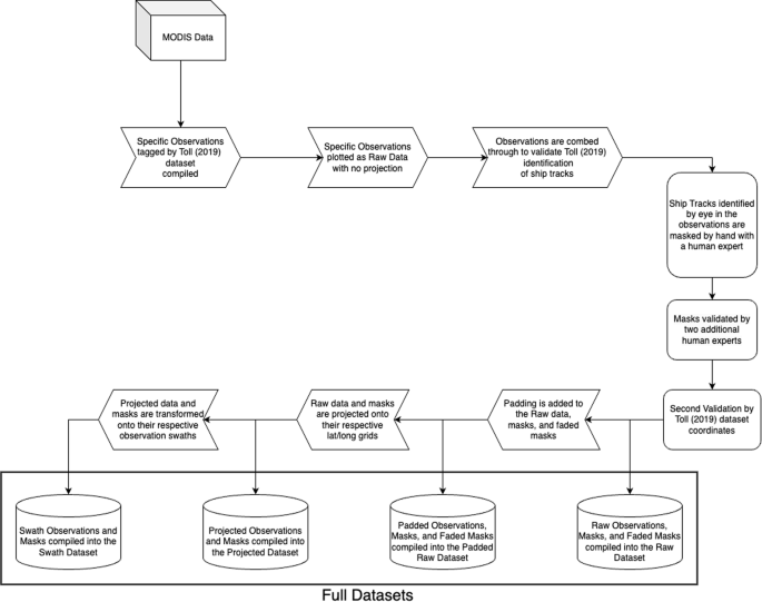
The full process of our proposed dataset creation from initial masking to the compilation of the various datasets we provide.

We use the datasets of^20,21,38 to validate our ship track masks and labelling methodology. More details about the validation process are provided in the Technical Validation section.

Methods

The first 300 MODIS observations identified in the 2019 dataset of²⁰ were collected from NASA’s Earth Data repository. All pixels containing ship tracks in these images were subsequently hand labelled. These masked images are presumed to be similar to the training data utilised in^23,24,26,36, though the masked images from those datasets are not publicly available.

Data Acquisition

The satellite data used in this dataset was acquired from NASA’s Earth Data repository and are MODIS data collected from the Aqua satellite. The MODIS instrument is one of several instruments carried by NASA’s Aqua and Terra satellites, providing large public quantities of data indirectly measuring atmospheric (aerosol) composition, cloud properties, atmospheric dynamics, ocean surface properties, and land features. For example, the MODIS-derived MYD06_L2 cloud product⁴² (MYD06_L2 specifies Level 2 data derived from cloud analysis from the Aqua platform), providing information on cloud properties such as cloud cover, top temperature and optical thickness, has been used to study cloud responses to aerosol injection from ship tracks and other pollution sources^36,37,43,44. In this paper, the MODIS MYD06_L2 calibrated radiances product is demonstrated to produce ship track labels/image masks. MYD06_L2 provides provides calibrated and geolocated at-aperture radiance measurements across 36 different spectral bands ranging from the visible to the infrared spectrum, and captures satellite-observed ship track presence. Such solar reflectance data are obtained in a 2000 km swath with the 36 spectral bands ranging from 0.4 μm to 14.4 μm generating 288 high quality images daily. Within each of these images ship tracks can be identified through their unique shapes and radiance signatures, which appear in images via different radiances in each spectral band. Built off raw data collected from the MODIS instrument, the L2 Cloud package is a dataset released by NASA that uses post processing algorithms devised after the Aqua satellite was launched to enhance and augment the data that MODIS collects⁴⁵. It is freely available for download under the MYD06-L2 directory in the Earth Data repository⁴⁵.

From this package, the Atmospherically Corrected Reflectance (Atm-Corr-Refl) data-field, which is known for high observability of ship tracks^23,25, was used for hand-labelling the ship tracks. Atm-Corr-Refl was calculated by NASA prior to its upload to the repository by post-processing of the raw MODIS data at the instrument’s 1 km resolution. The differences in cloud droplet sizes within the ship tracks when compared to surrounding clouds result in different reflectivites and thus distinct patterns in images produced using Atm-Corr-Refl, making it an attractive data product for identifying ship tracks. This distinctiveness is one reason for its use in previous datasets and its selection for this study.

Data Labelling

The image labels are masks of the Atm-Corr-Refl images. The images produced from Atm-Corr-Refl data were saved and manually labelled using GIMP⁴⁶, an open-source photo editing software. Specifically, the Free Select Tool was used to trace, extract, and mask ship tracks from the surrounding image. Figures 1 and 5(a) show the raw Atmospherically Corrected Reflectance for a single MODIS observation.

Fig. 5

Raw observation (a) and masked ship track images (b) of the Atm-Corr-Refl data taken July 15 2007 at 2:20 am in the North Pacific ocean, North East of Japan. Tracks visible in the raw image are then outlined and masked in (b) with the inter-track pixels preserved.

Masking refers to creating an accompanying image raster of the raw image, where everything that is not a ship track is blank, and only the ship tracks themselves are preserved. To produce the image masks, we identified ship track pixels by their distinct features: hollow polygonal, thin, and elongated patterns that frequently showed cloud convection⁴⁷. An emission point, or the head of a ship track, was defined as the thinner, more distinct starting point of the track relative to its elongated structure. This point was typically identified by an increase in brightness or albedo, indicating a higher concentration of smaller cloud droplets from ship exhaust. Tracks that were diffused fully into existing clouds, could not be distinguished from natural features, or were faint owing to lower reflectances, were ignored to avoid high occurrences of false positive observations (i.e., pixels erroneously labelled as ship tracks). For example, linear features along large cloud boundaries that lacked a clear emission point or a quasi-linear structure were excluded (see Fig. 1). Such features can arise from cirrus clouds²⁶ at higher altitudes or from sea-ice boundaries at high latitudes, neither of which produce the reflectivity changes characteristic of ship tracks. By focusing on clear emission points, higher albedo, and hollow polygonal patterns, we minimised false positives and achieved greater accuracy even under challenging conditions. Furthermore, our labelling strategy leveraged attributes highlighted by²⁶, whose algorithm successfully identifies ship tracks in cirrus-dense regions by emphasising these defining properties.

As emphasised, minimising false positives was a critical consideration for training high-quality machine learning models. We further ensured that tracks with visible though partially diffuse edges, as well as smaller or newly forming tracks, were labelled to capture a range of ship track types. Additionally, because many tracks form together in high-traffic shipping lanes^48,49,50 and can curve in unison while crossing bands of weaker cloudiness⁴⁷, we were careful to label multiple connected or curved structures simultaneously.

A common source of potential false positive tracks were linear features on the boundaries of large clouds. These often appeared near image edges or over regions with no clouds. If they lacked a well-defined head and blended into the ambient cloud field, we did not label them as ship tracks. Finally, if a track passed through a gap in cloud cover and then reappeared, we excluded the indeterminate gap region unless it exhibited a continuous structure.

All three labellers masked each image in two rounds. In the first round, obvious ship tracks were traced in GIMP using the Free Select Tool and placed on a black background. In the second round, each labeller inspected the data for faint or small ship tracks missed initially. A pixel was accepted as a track if at least two labellers labelled it. Although about 20–30% of tracks involved disagreement (mainly due to faint scenes), this consensus method reduced false positives, especially along track edges. This approach also helped capture both prominent and subtle ship tracks, ensuring minimal personal bias in distinguishing cloud from track. Figure 6 shows the labelling steps for one MODIS scene, including the final masked products.

Fig. 6

Raw Atm-Corr-Refl data, faded labelling, and masked labelling captured by the Aqua satellite at 9:15 pm on April 2nd, 2007, off the south coast of California.

While head identification was part of our manual labeling, we also augmented the dataset with automatically generated track statistics, namely the centreline and head of each labeled ship track. To do so, we deployed a skeletonisation algorithm to extract a one-pixel-wide centreline, then performed segment extraction and automated head detection using local wind data. This method provided a more detailed analysis of individual tracks in the masked images, particularly aiding the characterisation of fragmented, curved, or overlapping tracks.

Specifically, for each binary track mask, we first computed the skeleton via morphological thinning⁵¹, thereby preserving connectivity and topology in a one-pixel-wide centreline. The skeleton was then represented as a graph, with each pixel serving as a vertex and edges connecting adjacent pixels. We identified endpoints (pixels with a single neighbor) and junctions (pixels with more than two neighbors), and subsequently segmented the skeleton into independent paths by traversing from each endpoint through intermediate pixels (those with exactly two neighbors) until reaching another endpoint.

Due to the nature of labeled ship tracks, however, the skeletonisation process introduced fragmentation between single tracks due to noise, image artifacts, or overlapping cloud features, highlighting that continuous ship tracks could be broken into multiple identified segments. Thus, we merged segments to reconstruct the full track when the gap between an endpoint of one segment and an endpoint of an adjacent segment was small, and the angle at which the segments were directed was aligned, ensuring that separate segments were joined to become continuous-like track features.

Specifically, we merged two segments if the Euclidean distance between an endpoint k_i ∈ {1, 2} from one segment i (denoted ${{\bf{e}}}_{{k}_{i}}\in {{\mathbb{R}}}^{2}$) and an endpoint k_j ∈ {1, 2} from another segment j (denoted ${{\bf{e}}}_{{k}_{j}}\in {{\mathbb{R}}}^{2}$):

$$d({{\bf{e}}}_{{k}_{i}},{{\bf{e}}}_{{k}_{j}})=\parallel {{\bf{e}}}_{{k}_{i}}-{{\bf{e}}}_{{k}_{j}}{\parallel }_{2}$$

fell below a threshold of ten pixels, and if the cosine similarity between their local angles

$$\cos \theta =\cos ({\theta }_{{k}_{i}}-{\theta }_{{k}_{j}})$$

exceeded a threshold of 0.9. Here, each endpoint e_k of a segment k is associated with a scalar angle θ_k ∈ [0, 2π], which defines the local orientation of the centreline at that endpoint, and was computed over a short segment of pixels lying on the segment’s centreline near the endpoint.

Consequently, once the segments were merged into a continuous track, we determined the head of each fully merged track by comparing its new endpoints relative to the prevailing wind direction θ_W at the boundary layer, obtained from the fifth generation European Centre for Medium–Range Weather Forecasts (ECMWF) reanalysis data⁵². Letting ${{\bf{e}}}_{1},{{\bf{e}}}_{2}\in {{\mathbb{R}}}^{2}$ denote the two endpoints of a track, we first computed their local angles θ₁, θ₂ ∈ [0, 2π]. To account for the advection process that aerosols undergo after injection, the endpoint whose direction was least aligned with the wind (i.e., that with the smallest cosine similarity with θ_W) was therefore selected as the track head:

$${{\bf{e}}}^{\ast }=\mathop{\arg \,\min }\limits_{i\in \{1,2\}}\,\cos ({\theta }_{i}-{\theta }_{W}).$$

This approach not only identifies the track head but also provides metadata statistics (e.g., head position, centreline geometry, and alignment angles) that facilitate further plume-spreading behaviour analyses.

Last, although this algorithm proved valuable in determining the majority of track heads (see Fig. 7), a small number of cases (≈5% of labelled tracks) such as very short or curved tracks occasionally resulted in misidentified heads (e.g., a single-pixel track may have its head placed mid-segment rather than visually at an endpoint). Since our primary goal was to generate robust ship track masks, these head annotations are provided as metadata track statistics and should be interpreted with caution or refined further if high-precision head positioning is required.

Fig. 7

Example output of the skeletonisation and head detection process on a ship track from an Atm-Corr-Refl image (July 17, 2006, 2:16 pm). Left: Projected track mask. Center: Merged skeleton segments with identified endpoints (blue). Right: Calculated track heads (red).

Data Records

The dataset includes four categories of image data (in .png format) as well as additional track statistics (metadata).

The first category is full-sized; these contain both raw and masked images plotted in a large 1354 × 2030 size with no padding.

The second category is padded: Here, the images are plotted in raw format and are centred and padded to a size of 690 by 1000 pixels, which maintains the proportions of the original data without altering the image resolution or coarse-graining. This padding allows for seamless use in image manipulation functions, such as image convolution, without loss of data.

The padded category contains both the masked and faded images, which are saved in the same folder for ease of use in applications that require consistent image dimensions.

The third category is projected. These images are resampled onto a uniform and rectangular latitude/longitude grid through the Plate Carrée map projection to accurately represent the latitude and longitude coordinates. This category allows for better analysis of location-based information as the data more accurately reflects the geospatial area it was collected over.

An issue with this projected approach is that some pixel values from the MODIS instrument are missing or corrupted. To correct for these, we created two further subsets of the projected category for visualisation purposes: interpolated and minimum, corresponding to missing values either being interpolated from the image or imputed using the minimum non-missing pixel intensity found in each image. We found that ship tracks can be highlighted more strongly in the interpolated images, though for climate analysis, the minimum version is recommended as it is less likely to generate false positives or represent swaths of missing data as a cloud feature. This ensures that the dataset is comprehensive and usable for various analyses.

The final category is swath: these are the images plotted using the actual latitude and longitude of each pixel, without resampling onto a uniform grid. These images accurately reflect the satellite’s swath path over the Earth’s surface, accounting for the curvature of the Earth. In contrast, the raw images are plotted directly from the data array without considering the geolocation of each pixel, resulting in rectangular images that may appear distorted or squeezed at the edges due to the Earth’s curvature not being taken into account. A swath example is shown in Fig. 1b.

The naming of the files within each directory follows the convention YearDay-Time-Category.png, which is inherited from the NASA Earth Data repository where the original files are hosted. Here, the Category is either Raw, Masked, or Faded, corresponding to the raw reflectance images, pixels of ship tracks, and faded images, respectively. As an example, a raw reflectance image taken on Day 166 in 2006 at 18:50 is named 2006166-1850-Raw.png. For further use of this dataset, images composed by other spectral reflectance bands 0.65 μm, 0.86 μm, 1.2 μm, and 1.6 μm can be easily extracted using the available masks.

The first class of images is the Atmospherically Corrected Reflectance data from the MODIS instrument. Since this data is initially attained in packed (raw) format, the images were first parsed to obtain the actual (unpacked) values of the reflectances. This conversion process is determined by the offset and scale factors that are provided through the L2 data package and are inherent to the raw (.hdf) format of the MODIS data.

In the raw images, the data is plotted directly from the data array without considering the geolocation of each pixel. This results in rectangular images of size 1354 x 2030 that may appear distorted or squeezed at the edges due to the Earth’s curvature not being taken into account.

The second class of images is the masked data. This is the data where only the pixels comprising a ship track are non-zero, with all other pixels set to zero. We note that the ship track pixels are unaltered and retain their original pixel values. These images are labelled in each directory appropriately.

Finally, the last class of images, saved only in the padded directory, are the faded images. This dataset was produced solely for visualisation purposes, in order to show the ship track labels in the context of the full image.

The use case for this data is for understanding and display of the masking, as is shown in Fig. 6. In these images, which serve as a step between the raw images and the masked images, all non-ship track pixels are reduced to 50% transparency, while the ship track pixels remain unaltered. This fading of the background or surrounding clouds allows for better visualisation of the ship tracks themselves for presentation or validation of correct masking. Just as with the masked images, these images have no alterations on the ship track pixels; only the non-ship track pixels are altered.

Additionally, we augment the dataset with automatically generated track statistics: the centreline and head for each labelled ship track as described previously. These metadata are stored in JSON format as nested dictionaries, with each track represented by keys including “head_lat”, “head_lon”, “head_angle”, and “wind_angle”. Here, “head_lat” and “head_lon” denote the spatial coordinates of the track head, while “head_angle” is defined as the average angle in degrees (with North as 0^∘) between points along the centreline and the identified head. The “wind_angle” represents the average wind direction across the centreline points, differing by approximately 180^∘ from the head angle to be consistent with the wind advecting the aerosol track from its head.

A summary of the dataset components, including types, categories, contents (classes) and intended usages is shown in Table 1.

Table 1 Summary of dataset components, dimensions, and contents.

Technical Validation

To ensure the validity of our labelled ship tracks, we compared our dataset⁴⁰ with pre-existing ship track databases. Ideally, validation would involve verifying each ship track against the presence of a ship, as recorded by the Automatic Identification System (AIS). However, since AIS data from before 2009 is not available, our validation relies on quantitative comparisons with the other human and machine-labelled ship track databases discussed in this paper. In an ideal classification problem, validation would comprise of identifying:

• True positives (TP): Correctly identified ship tracks.

• False positives (FP): Incorrectly identified ship tracks.

• False negatives (FN): Missed true ship tracks.

Defining a true negative in this study is not meaningful since all datasets only present labelled (and not unlabelled) ship tracks. Thus, due to the nature of the dataset, only false positives, true positives, and false negatives can be analysed.

The technical validation for this dataset is split into three parts. The first two parts utilise the hand-labelled 2019 dataset of²⁰, as the source of the direct comparison with existing data. Due to large amounts of apparent false negative tracks, i.e. true ship tracks that were incorrectly unlabelled in the dataset of²⁰, as demonstrated via comparisons between the 2022 datasets^21,38 and seen in Fig. 1, the last two validation pieces subsequently invoke comparisons with the coordinate²¹ and polygon³⁸ datasets. We opt not to show comparisons between our dataset⁴⁰ and the machine labelled dataset of²², since it is directly derived from the raw 2022b hand-labelled dataset of³⁸, which contains the track labels over the time period we study.

The images used to produce our dataset⁴⁰ were selected using the corresponding dates and times of ship track labels present in the 2019 dataset²⁰. Thus, the images used to produce our dataset were all presumed to have ship tracks present before they were hand-labelled/masked. However, among these images, a number were removed, as they had no discernible tracks. The validation was conducted after the masking was completed, by comparing the latitude/longitude coordinates along the track centrelines, as listed in²⁰, with those masked and pre-filtered by the our dataset labels. This procedure was performed to validate that the correct features within each image were masked. To do so, the swath data was projected onto a latitude/longitude grid at 0.001 degree resolution, equivalent to a pixel at approximately 0.01 km spacing. Ship track pixels were then matched with sinusoidal projected coordinates identified by²⁰. In doing so, we find that our labelled tracks recover 100% of the previously identified tracks in²⁰. Further we find that the ship track pixels in our dataset contain 100% of the centreline coordinates of ship tracks in²⁰. Although this analysis confirms that our labels are in agreement with those found previously, we found multiple discrepancies in that for several images analysed in the 2019 dataset²⁰, both our labels and the labels of²¹ identify multiple ship tracks, while the labellers of^20,38 only identify a subset of these.

A qualitative visual assessment of the similarity between unlabelled linear features and labelled ship tracks was thus preliminarily conducted. Figure 8 shows an example of three ship tracks that we⁴⁰ and the dataset of²¹ label, in which only two are labelled in the datasets of²⁰ and³⁸.

Fig. 8

Raw Atm-Corr-Refl data at 6:45 pm on June 15th 2006 off the coast of Chile, plotted as a swath with all track labels from all existing datasets (a). Projected images, zoomed in on ship tracks. Tracks shown are projected and unlabelled (b) and with the validated ship tracks (c). Origin points of tracks tagged in^20,38 are marked in red, while the unlabelled track (labelled both by the proposed⁴⁰ and²¹ datasets) is marked in orange.

To better understand the accuracy of our dataset and quantify the apparent false negatives in²⁰, we last utilise the datasets^21,38 that consist of a central coordinate²¹, or a polygon region around the centreline³⁸ of all labelled ship tracks in the time period we study. With each dataset (taken to be “ground-truth”), we compare the “ground-truth” labels and their locations with respect to our ship track pixel masks. Specifically, we use a buffer of 5 pixels (or 0.05 km) equivalent to an average of 1 standard deviation of a track’s half-width in line with²⁴, to account for slight differences in labelling and determined locations, surrounding each of our track’s labelled pixels. In doing so, we study if at least one track coordinate (from “ground-truth” datasets^20,21), or centreline polygon area coordinate (from “ground-truth” dataset³⁸) lies in in this buffer. The number of “ground truth” tracks that do not lie in this zone, and the number of “ground-truth” tracks not belonging to one of these areas are also measured.

For each track, a true positive (denoted TP), i.e. a ship track labelled by the “ground-truth” dataset that is also labelled by us, is determined for every label from the “ground-truth” dataset (coordinates or centreline polygon) that can be matched within a track we label. A false positive (denoted FP) is determined if a track we label as a ship track, cannot be matched to a label from the “ground truth” dataset. A false negative (denoted FN) is determined if a label presented in the “ground truth” dataset cannot be matched to a track we label. By counting the number of true positives (#TP), false positives (#FP) and false negatives (#FN) between a dataset and the “ground-truth” dataset, standard comparative metrics, namely the precision, recall and F1 scores (a metric which combines both precision and recall into a single score), defined by

$$\,{\rm{Precision}}\,=\frac{\#TP}{\#TP+\#FP},\quad \,{\rm{Recall}}\,=\frac{\#TP}{\#TP+\#FN},\quad {F}_{1}=2\cdot \frac{{\rm{Precision}}\cdot {\rm{Recall}}}{{\rm{Precision}}+{\rm{Recall}}},$$

can be calculated.

In this context, the precision metric measures the proportion of true ship tracks among all tracks labelled as ship tracks. Recall, on the other hand, assesses labelling ability to find all true tracks in a given image. High recall measures how well labels capture true ship tracks, without leaving too many behind. The F₁ score balances both the precision and recall to provide an overall performance measure. It indicates how well the labelling procedure correctly labels true ship tracks and ignores false tracks, thus providing a balanced view of the overall performance of a labelled dataset. Precision, recall, and the F₁ score are all range between 0 and 1 (inclusive), with higher scores closer to 1 indicating better performance. We calculate these metrics between our proposed dataset and the three existing datasets^20,21,38, and also between all pairs of these existing datasets. These metrics are shown in Table 2.

Table 2 Table showing the precision, recall and F₁ scores between the proposed dataset and three existing ship track datasets.

The results of this analysis show a high level of variation between our dataset⁴⁰ and the existing datasets of^20,21,38 but also considerable disagreement between the presently existing datasets. In addition to providing the F₁ score for our dataset⁴⁰ against the three “ground-truth” datasets, Table 2 shows the F₁ scores of the validation datasets against each other. It is shown here that the dataset providing the most agreement with our dataset is the dataset of²¹, with an F₁ score of 58%. While the other F₁ scores are lower at 34%, this is still shown to be higher than comparing the datasets of^20,38 against the “ground-truth” dataset of²¹ at 23%. These results indicate that our dataset tends to label more tracks than^20,38, but fewer than that of²¹, indicating a potentially higher number of false positives (i.e. many labelled false ship tracks) in the dataset of²¹, and a higher number false negatives (i.e. many unlabelled true ship tracks) in the datasets of^20,38.

The exception to our analysis arises from the comparison between the 2019 dataset²⁰ and the 2022b dataset³⁸, which has the highest F₁ score of 63% and similar precision and recall scores at the same value. This is not surprising, however, since both datasets are derived from the same unpublished ship track dataset, first mentioned in³⁴, rendering the datasets^20,38 non mutually exclusive. Further, while it remains unclear whether the large subset of unlabelled tracks in these datasets (against that of our data⁴⁰ and²¹) were intentionally excluded or inadvertently missed during the original labelling process, we note that these datasets rely strictly on identifying a clear head for track confirmation³⁴ as opposed to other identifying track features, which may additionally explain the disparities in the resulting precision and recall values.

Our overall validation process emphasises that while our dataset details tracks that are consistent with existing datasets, it also captures additional tracks missed by others. This highlights the need for careful consideration of both false positives and negatives in ship track labelling, and its potential impact in training a more robust classification algorithm for automating track identification.

Usage Notes

The images in this dataset was created and managed using Python and its PIL image module⁵³. The additional track endpoints, heads and centrelines are provided as longitude/latitude coordinates and angles from North, that can be used in conjugation with the rasters, to identify specific track regions. This dataset primarily serves to be used as training data for supervised machine learning, or as a raster dataset for the analysis of ship track or surrounding climate behaviour in the given period. As such, the raw images and masked track images are the ones recommended to use, with the faded images only for use in visualisation or to reference where the ship tracks lay within the broader context of the image. Specific usage of our dataset⁴⁰ per data directory is depicted in Table 3.

Table 3 Table showing the utility of each sub-dataset contained in our proposed full dataset for visualization, masking, validation and supervision in Machine Learning (ML) algorithms.

References

Hoffmann, F. & Feingold, G. Cloud microphysical implications for marine cloud brightening: The importance of the seeded particle size distribution. Journal of the Atmospheric Sciences 78(10), 3247–3262 (2021).
Albrecht, B. A. Aerosols, Cloud Microphysics, and Fractional Cloudiness. Science 245, 1227–1230, https://doi.org/10.1126/science.245.4923.1227 (1989).
Diamond, M. S., Director, H. M., Eastman, R., Possner, A. & Wood, R. Substantial cloud brightening from shipping in subtropical low clouds. AGU Advances 1(1), e2019AV000111, https://doi.org/10.1029/2019AV000111 (2020).
Latham, J. Control of global warming? Nature 347(6291), 339–340, https://doi.org/10.10384/347339b0 (1990).
Wood, R. Assessing the potential efficacy of marine cloud brightening for cooling Earth using a simple heuristic model. Atmospheric Chemistry and Physics 21(19), 14507–14533 (2021).
Yuan, T. et al. Abrupt reduction in shipping emission as an inadvertent geoengineering termination shock produces substantial radiative warming. Communications Earth & Environment 2, 195, https://doi.org/10.1038/s43247-021-00248-x (2021).
Wan, J. S., Fasullo, J. T., Rosenbloom, N., Chen, C.-C. J. & Ricke, K. Targeted marine cloud brightening can dampen El Niño, arXiv preprint arXiv:2406.07853 (2024).
Zhang, J., Chen, Y.-S., Gryspeerdt, E. & Yamaguchi, T. Large radiative forcing from the 2020 shipping fuel regulation is hard to detect. Communications Earth & Environment 6(1), 18.
Chen, Y. et al. Substantial cooling effect from aerosol-induced increase in tropical marine cloud cover, Nature Geoscience, 1–7 (2024).
Mülmenstädt, J. & Feingold, G. The radiative forcing of aerosol–cloud interactions in liquid clouds: Wrestling and embracing uncertainty. Current Climate Change Reports 4(1), 23–40 (2018).
Intergovernmental Panel on Climate Change (IPCC), Clouds and Aerosols, in Climate Change 2013 - The Physical Science Basis: Working Group I Contribution to the Fifth Assessment Report of the Intergovernmental Panel on Climate Change, Cambridge University Press, Cambridge, 571–658 (2014).
Twomey, S. The nuclei of natural cloud formation part II: The supersaturation in natural clouds and the variation of cloud droplet concentration. Geofisica pura e applicata 43(1), 243–249, https://doi.org/10.1007/BF01993560 (1959).
Sorooshian, A. et al. Spatially coordinated airborne data and complementary products for aerosol, gas, cloud, and meteorological studies: the NASA ACTIVATE dataset. Earth System Science Data 12, 123–134, https://doi.org/10.5067/SUBORBITAL/ACTIVATE/DATA001 (2020).
Tang, S. et al. Understanding Aerosol-Cloud Interactions in a Single-Column Model: Intercomparison with Process-Level Models and Evaluation against ACTIVATE Field Measurements, EGUsphere, https://doi.org/10.5194/egusphere-2023-3149 (2023).
Favelle, C. To Slow Global Warming, Scientists Test Solar Geoengineering, The New York Times, https://www.nytimes.com/2024/04/02/climate/global-warming-clouds-solar-geoengineering.html (2024).
Wood, R. & Ackerman, T. P. Defining success and limits of field experiments to test geoengineering by marine cloud brightening. Climatic Change 121, 459–472 (2013).
Harrison, D. P. An Overview of Environmental Engineering Methods for Reducing Coral Bleaching Stress, in Oceanographic Processes of Coral Reefs, 403–418, CRC Press (2024).
Sovacool, B. K., Baum, C. M., Low, S. & Fritz, L. Coral reefs, cloud forests and radical climate interventions in Australia’s Wet Tropics and Great Barrier Reef. PLOS Climate 2(10), e0000221 (2023).
Pattyn, C. A. et al. Sub-grid scale mixing of injected particulate and a cloud-like aerosol in a laboratory environment, Forthcoming, (2024).
Toll, V. & Bellouin, N. Polluted cloud tracks detected in MODIS satellite images, University of Reading, https://doi.org/10.17864/1947.208 (2019).
Song, H. Datetimes and Locations of ship-tracks (Version 1), Harvard Dataverse, https://doi.org/10.7910/DVN/JII4DN (2022).
Watson-Parris, D., Laurenson, A. & Clewley, D. Ship tracks detected using machine learning algorithm (Version 1.0), Zenodo, https://doi.org/10.5281/zenodo.7038703 (2022).
Yuan, T. et al. Global reduction in ship-tracks from sulfur regulations for shipping fuel. Science Advances 8(29), eabn7988, https://doi.org/10.1126/sciadv.abn7988 (2022).
Watson-Parris, D. et al. Shipping regulations lead to large reduction in cloud perturbations. Proceedings of the National Academy of Sciences 119(41), e2206885119 (2022).
Segrin, Matthew S., Coakley, James A., and Tahnk, William R. MODIS Observations of Ship Tracks in Summertime Stratus off the West Coast of the United States, Journal of the Atmospheric Sciences, 64(12) (2007).
Yuan, T. et al. Automatically Finding Ship Tracks to Enable Large-Scale Analysis of Aerosol-Cloud Interactions. Geophysical Research Letters 46(13), 7726–7733, https://doi.org/10.1029/2019GL083441 (2019).
Twomey, S., Howell, H. B. & Wojciechowski, T. A. Comments on Anomalous Cloud Lines. Journal of Atmospheric Science 25, 333–334 (1966).
Myhre, G. et al. Climate Change 2013: The Physical Science Basis. Contribution of Working Group I to the Fifth Assessment Report of the Intergovernmental Panel on Climate Change, p. 1535 (2013).
McCoy, D. T. et al. The global aerosol-cloud first indirect effect estimated using MODIS, MERRA, and AeroCom. Journal of Geophysical Research: Atmospheres 122(3), 1779–1796, https://doi.org/10.1002/2016jd026141 (2017).
Liu, Q. et al. Modeling of Ship Effluent Transport and Its Sensitivity to Boundary Layer Structure. Journal of the Atmospheric Sciences 57(16), 2779–2791, https://doi.org/10.1175/1520-0469(2000)057<2779:MOSETA>2.0.CO;2 (2000).
Patel, L. & Shand, L. Toward data assimilation of ship-induced aerosol-cloud interactions. Environmental Data Science 1, e31, https://doi.org/10.1017/eds.2022.21 (2022).
Manshausen, P., Watson-Parris, D., Christensen, M. W., Jalkanen, J.-P. & Stier, P. Invisible ship tracks show large cloud sensitivity to aerosol. Nature 610, 101–106, https://doi.org/10.1038/s41586-022-05122-0 (2022).
Warburton, P., Shuler, K. & Patel, L. Deep Learning Aerosol-Cloud Interactions from Satellite Imagery. in Proceedings of the AAAI Symposium Series 2, 159–165 (2023).
Christensen, M. W. and Stephens, G. L. Microphysical and macrophysical responses of marine stratocumulus polluted by underlying ships: 2. Impacts of haze on precipitating clouds, Journal of Geophysical Research: Atmospheres, 117(D11), https://doi.org/10.1029/2011JD017125 (2012).
McMichael, L. A., Schmidt, M. J., Wood, R., Blossey, P. N. and Patel, L. Exploring ship track spreading rates with a physics-informed Langevin particle parameterization, EGUsphere, 2024, 1–33 (2024).
Toll, V., Christensen, M., Quaas, J. & Bellouin, N. Weak average liquid-cloud-water response to anthropogenic aerosols. Nature 572(7767), 51–55 (2019).
Toll, V., Christensen, M., Gassó, S. & Bellouin, N. Volcano and ship tracks indicate excessive aerosol-induced cloud water increases in a climate model. Geophysical Research Letters 44(24), 12–492 (2017).
Watson-Parris, D. Training data for ship track detection machine learning algorithms (Version 1.0), Zenodo, https://doi.org/10.5281/zenodo.7038715 (2022).
Chen, Y.-C. et al. Occurrence of lower cloud albedo in ship tracks. Atmospheric Chemistry and Physics 12(17), 8223–8235 (2012).
Warburton, P., Shuler, K. & Patel, L. Image masks of global ship tracks for NASA MODIS data products, Figshare, https://doi.org/10.6084/m9.figshare.24098517.v2 (2023).
Schreier, M., Mannstein, H., Eyring, V. & Bovensmann, H. Global ship track distribution and radiative forcing from 1 year of AATSR data, Geophysical Research Letters, 34(17), https://doi.org/10.1029/2007GL030664 (2007).
Platnick, S. et al. The MODIS cloud optical and microphysical products: Collection 6 updates and examples from Terra and Aqua. IEEE Transactions on Geoscience and Remote Sensing 55(1), 502–525 (2016).
Gryspeerdt, E. et al. Constraining the aerosol influence on cloud liquid water path. Atmospheric Chemistry and Physics 19(8), 5331–5347 (2019).
Gryspeerdt, E., Smith, T. W. P., O’Keeffe, E., Christensen, M. W. & Goldsworth, F. W. The impact of ship emission controls recorded by cloud properties. Geophysical Research Letters 46(21), 12547–12555 (2019).
Platnick, S. et al. MODIS Atmosphere L2 Cloud Product (06_L2). NASA MODIS Adaptive Processing System, Goddard Space Flight Center, USA, https://doi.org/10.5067/MODIS/MYD06_L2.061 (2015).
Lecarme, O. & Delvare, K. The book of GIMP: A complete guide to nearly everything, No Starch Press (2013).
Conover, J. H. Anomalous Cloud Lines. Journal of Atmospheric Science 23, 778–785, https://doi.org/10.1175/1520-0469(1966)023<0778:ACL>2.0.CO;2 (1966).
Durkee, P. A., Noone, K. J. & Bluth, R. T. The Monterey area ship track experiment. Journal of the Atmospheric Sciences 57(16), 2523–2541 (2000).
Coakley, J. A. Jr., Bernstein, R. L. & Durkee, P. A. Effect of ship-stack effluents on cloud reflectivity. Science 237(4818), 1020–1022 (1987).
Durkee, P. A. et al. Composite Ship Track Characteristics. Journal of the Atmospheric Sciences 57(16), 2542–2553 (2000).
Zhang, T. Y. & Suen, C. Y. A fast parallel algorithm for thinning digital patterns. Communications of the ACM 27(3), 236–239 (1984).
Hersbach, H. et al. ERA5 hourly data on pressure levels from 1940 to present, Copernicus Climate Change Service (C3S) Climate Data Store (CDS) [data set] (2018).
Umesh, P. Image Processing in Python, CSI Communications, 23 (2012).
Acknowledgements
We would like to thank Dr. Erika Roesler at Sandia National Laboratories for her subject matter expertise and independent review of this work for its scientific accuracy and clarity of exposition. We would also like to thank Prof. Rob Wood and Dr. Luke McMichael at the University of Washington for stimulating discussions of this topic, and their subject matter expertise. This paper describes objective technical results and analysis. Any subjective views or opinions that might be expressed in the paper do not necessarily represent the views of the U.S. Department of Energy or the United States Government. This work was supported by the Laboratory Directed Research and Development program at Sandia National Laboratories, a multimission laboratory managed and operated by National Technology and Engineering Solutions of Sandia, LLC, a wholly-owned subsidiary of Honeywell International, Inc., for both the U.S. Department of Energy’s National Nuclear Security Administration under contract DE-NA0003525.
Author information
Authors and Affiliations
Contributions
P.W., K.S. and L.P. conceived the experiments, P.W., K.S and L.P. conducted the experiments, P.W. and J.P.Z. analysed the results. All authors reviewed the manuscript.
Corresponding author
Ethics declarations
Competing interests
The authors declare no competing interests.
Additional information
Publisher’s note Springer Nature remains neutral with regard to jurisdictional claims in published maps and institutional affiliations.
Rights and permissions
Open Access This article is licensed under a Creative Commons Attribution-NonCommercial-NoDerivatives 4.0 International License, which permits any non-commercial use, sharing, distribution and reproduction in any medium or format, as long as you give appropriate credit to the original author(s) and the source, provide a link to the Creative Commons licence, and indicate if you modified the licensed material. You do not have permission under this licence to share adapted material derived from this article or parts of it. The images or other third party material in this article are included in the article’s Creative Commons licence, unless indicated otherwise in a credit line to the material. If material is not included in the article’s Creative Commons licence and your intended use is not permitted by statutory regulation or exceeds the permitted use, you will need to obtain permission directly from the copyright holder. To view a copy of this licence, visit http://creativecommons.org/licenses/by-nc-nd/4.0/.
About this article
Cite this article
Warburton, P., Shuler, K., Zenker, J.P. et al. Image masks of global ship tracks for NASA MODIS data products. Sci Data 12, 1060 (2025). https://doi.org/10.1038/s41597-025-04911-2
Received:
Accepted:
Published:
Version of record:
DOI: https://doi.org/10.1038/s41597-025-04911-2